Class 4 (Systems: Their Properties)

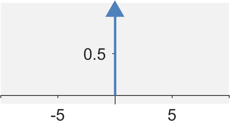
Impulse functions

The Dirac $\delta$ signal (continuous-time impulse signal) is defined by $$ \delta(t) = \left\{ \begin{eqnarray} \infty &\quad& \textrm{for} \quad t = 0 \\ 0 &\quad& \textrm{for} \quad t \neq 0 \end{eqnarray} \right. $$ where $$\int_{-\infty}^{\infty} \delta(t) dt = 1 $$

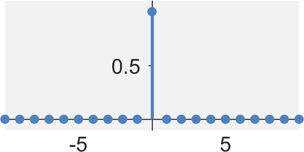
The Kronecker $\delta$ signal (discrete-time impulse signal) is defined by $$ \delta[n] = \left\{ \begin{eqnarray} 1 &\quad& \textrm{for} \quad n = 0 \\ 0 &\quad& \textrm{for} \quad n \neq 0 \end{eqnarray} \right. $$

The properties of impulse signals:

• Energy: $E_{x} = \textrm{not well defined}$
• Power: $P_{x} = 0$
• Even / Odd?: Even (Understanding why is beyond the purview of this course. You will not be tested on this.)
• Periodic?: No
• Causal?: Yes

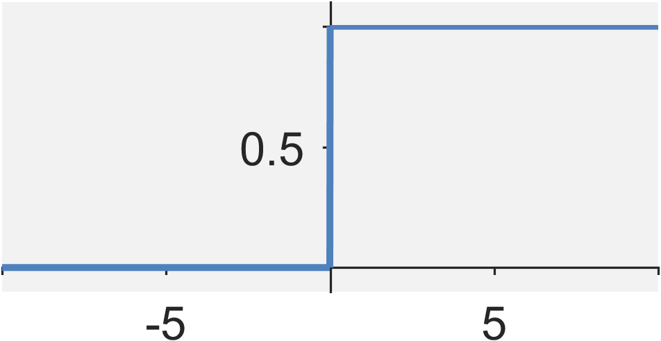
Heaviside step functions

The continuous-time step function $u(t)$ is defined by $$ u(t) = \int_{-\infty}^{t} \delta(\tau) d\tau = \left\{ \begin{eqnarray} 1 &\quad& \textrm{for} \quad t \geq 0 \\ 0 &\quad& \textrm{for} \quad t < 0 \end{eqnarray} \right. $$

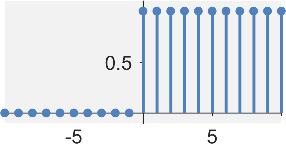
The discrete-time step function $u[n]$ is defined by $$ u[n] = \sum_{k = -\infty}^{n} \delta[k] = \left\{ \begin{eqnarray} 1 &\quad& \textrm{for} \quad n \geq 0 \\ 0 &\quad& \textrm{for} \quad n < 0 \end{eqnarray} \right. $$

The properties of the Heaviside step functions:

• Energy: $E_{x} = \infty$
• Power: $P_{x} = 1/2$
• Even / Odd?: Neither
• Periodic?: No
• Causal?: Yes

Cosines and sines

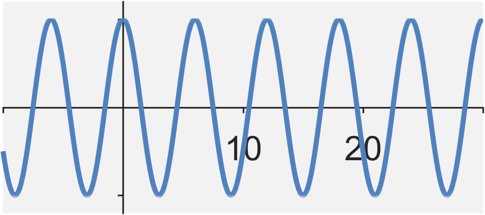
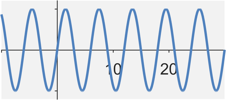
The continuous-time cosine and sine signals are defined by $$ x_1(t) = \cos(\omega_0 t) \quad , \quad x_2(t) = \sin(\omega_0 t) $$

The properties of the continuous-time cosines or sines:

• Enegry: $E_{x} = \infty$
• Power: $P_{x} = 1/2$
• Even / Odd?: $\cos(\omega_0 t)$ is even and $\sin(\omega_0 t)$ is odd
• Periodic?: Yes
• Fundamental frequency: $f_0 = \omega_0/(2 \pi)$
• Fundamental period: $T_0 = 1/f_0$
• Causal?: No

Stepped exponential

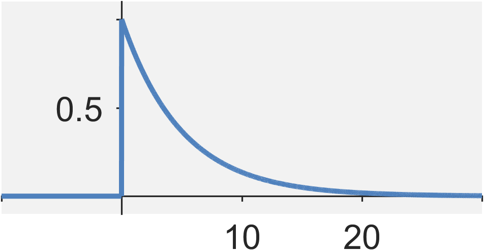
A continuous-time exponential signal is defined by $$ x(t) = e^{a_0 t} u(t) $$

The properties of the exponential signals are:

• Enegry: $E_{x} = \left\{ \begin{eqnarray} \infty &\quad& \textrm{for} \quad a_0 \geq 0 \\ - 1/(2 a_0) &\quad& \textrm{for} \quad a_0 < 0 \end{eqnarray} \right.$
• Power: $P_{x} = 0$
• Even / Odd?: No
• Periodic?: No
• Causal?: Yes

Complex exponentials

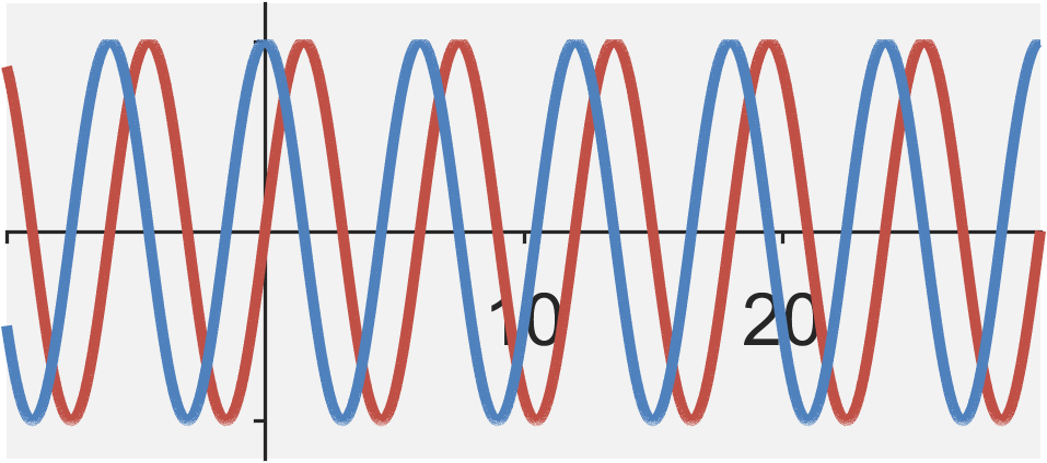
The continuous-time complex exponential signal is defined by $$ \begin{eqnarray} x(t) &=& e^{(j \omega_0 + a_0)t} \\ &=& \cos(\omega_0 t) + j \sin(\omega_0 t) \end{eqnarray}$$

The properties of the continuous-time complex exponential:

• Enegry: $E_{x} = \infty$
• Power: $P_{x} = 1$
• Even / Odd?: No, but its components are: $\cos(\omega_0 t)$ is even and $\sin(\omega_0 t)$ is odd
• Periodic?: Yes
• Fundamental frequency: $f_0 = \omega_0/(2 \pi)$
• Fundamental period: $T_0 = 1/f_0$
• Causal?: No

Stepped general exponential

The continuous-time general exponential signal is defined by $$ \begin{eqnarray} x(t) &=& e^{(j \omega_0 + a_0)t} u(t) \\ &=& \left[ e^{a_0 t} \cos(\omega_0 t) + j e^{a_0 t} \sin(\omega_0 t) \right] u(t) \end{eqnarray}$$

The properties of the general exponential signals are:

• Enegry: $E_{x} = \left\{ \begin{eqnarray} \infty &\quad& \textrm{for} \quad a_0 \geq 0 \\ - 1/(2 a_0) &\quad& \textrm{for} \quad a_0 < 0 \end{eqnarray} \right.$
• Power: $P_{x} = 0$
• Even / Odd?: No
• Periodic?: No
• Causal?: Yes

Input-output system model

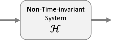
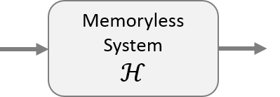
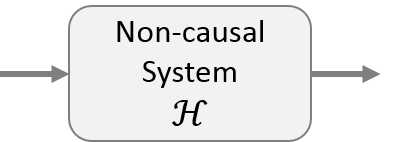
Throughout the course, we will visualize systems using block diagrams, such as the one below.

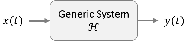
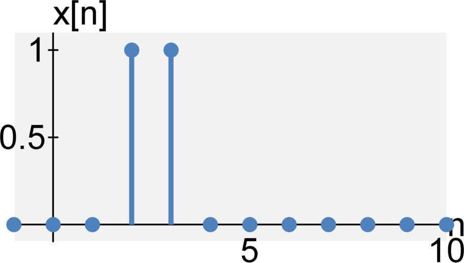
In this diagram, the $x(t)$ is the input, which the system manipulates, and $y(t)$ is the output. For general systems, we can represent a system by a function $\mathcal{H}\{ \cdot \}$ that operates on signals. Therefore the system above can be formally expressed as $$y(t) = \mathcal{H}\{ x(t) \}.$$ Note that this notation will disappear when we start focusing on linear, time-invariant in the next class.

Continuous-time or discrete-time

A continuous-time system whose inputs and outputs are continuous-time signals. A discrete-time system is one whose inputs and outputs are discrete-time signals.

Analog or digital

An analog system whose inputs and outputs are analog signals. A digital system is one whose inputs and outputs are digital signals.

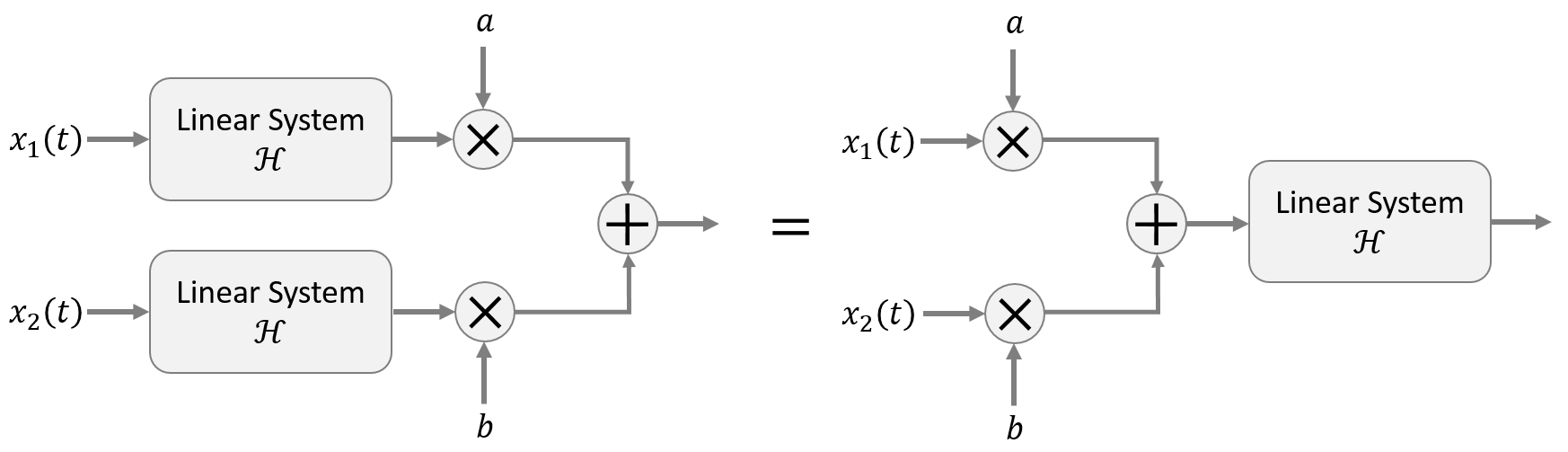
Linear or nonlinear

A system is linear if it obeys the law of superposition. Formally, if $\mathcal{H}\{ \cdot \}$ is a system with input $x_1(t)$ or $x_2(t)$ and output $y_2(t)$ or $y_1(t)$ such that $$y_1(t) = \mathcal{H}\{ x_1(t) \} \\ y_2(t) = \mathcal{H}\{ x_2(t) \} ,$$ then the system is linear if $$\begin{eqnarray} y(t) &=& \mathcal{H}\{ a x_1(t) + b x_2(t) \} \\ &=& a \mathcal{H}\{ x_1(t) \} + b \mathcal{H} \{ x_2(t) \} \\ &=& a y_1(t) + b y_2(t) , \end{eqnarray} $$ where $a$ and $b$ are arbitrary scalar numbers.

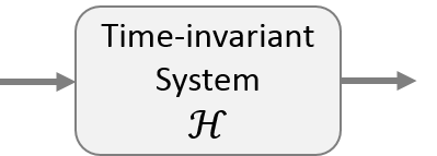
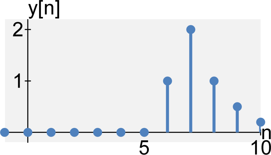
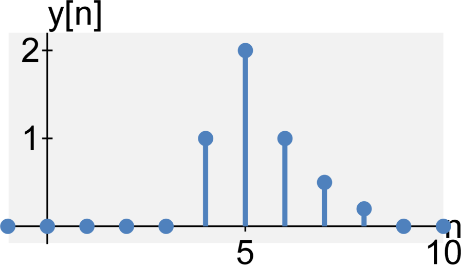
Time invariant or time varying

A system is time-invariant if the system does not change with time. Formally, if $\mathcal{H}\{ \cdot \}$ is a system at time $t$ with input $x(t)$ and output $y(t)$, such that $y(t) = \mathcal{H}\{ x(t)\}$, then the system is time-invariant if $$y(t + \tau) = \mathcal{H}\{ x(t + \tau) \} $$ for any arbitrary time delay $\tau$. That is, if we delay our input, we expect the output to be delayed by the same amount. In a time-invariant system, an input delay may not affect the output signal in any other way.

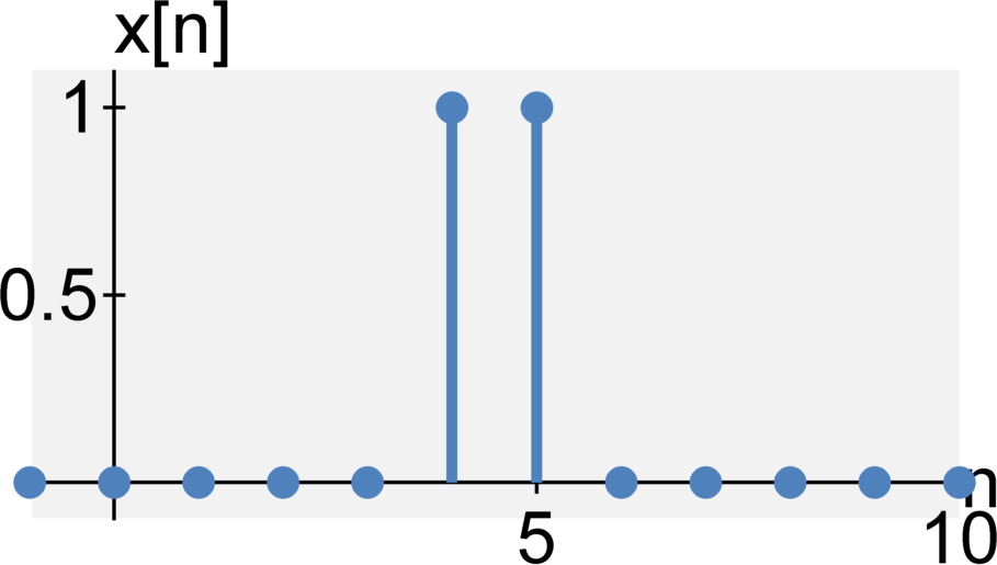
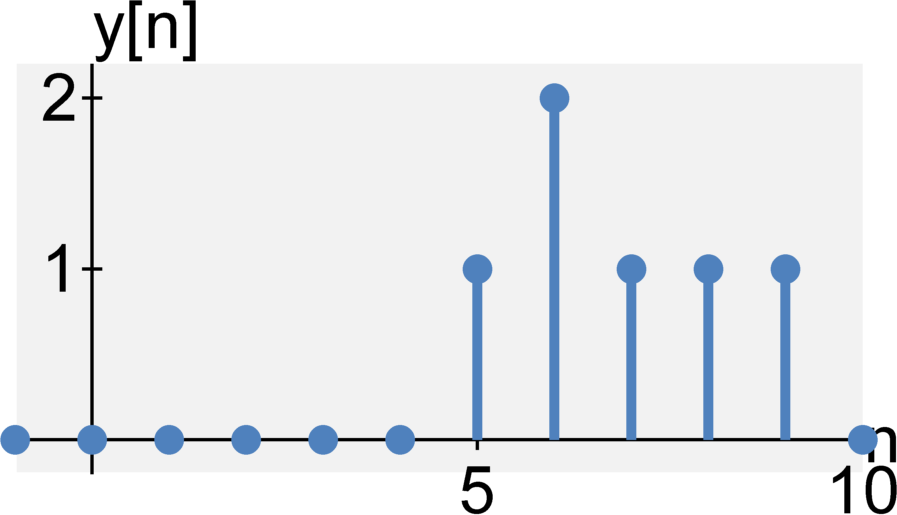
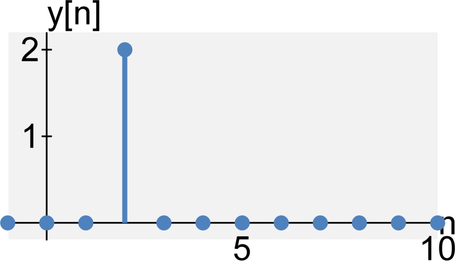
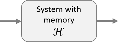
Memoryless or with memory

A system is instantaneous (or memoryless) if its output at time $t$ only depends on the input at time $t$. A system is dynamic (or has memory) if the output on $t$ depends on the input at time $t$ and any previous inputs $t - \tau \quad \textrm{for} \quad \tau > 0$. That is, the system "remembers" previous inputs.

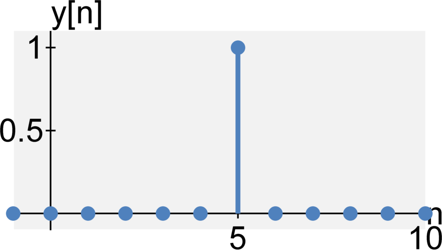
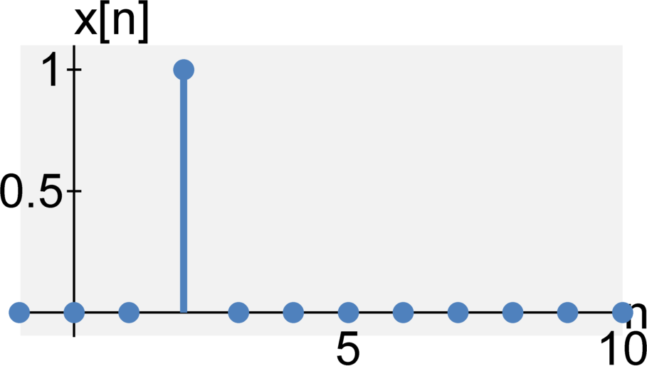
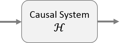
Causal or non-causal

A system is causal (or physical or non-anticipative) if its output at time $t$ only depends on the current input at time $t$ and its past outputs at time $t - \tau \quad \textrm{for} \quad \tau > 0$. Hence, the output does not depend on future inputs.

All real-time systems are causal systems.

Bounded-input, bounded-output (BIBO) stable or unstable

A system is BIBO stable if any amplitude-bounded input (i.e., the signal $x(t)$ never reaches or approaches $\infty$ for all $t$) yields and amplitude-bounded output (i.e., the signal $y(t)$ never reaches or approaches $\infty$ for all $t$).

Note that there are many different types of stability criteria for systems. We will discuss stability in much greater detail after learning about the Laplace transform.