Class 15 (The Laplace Transform)
Motivation
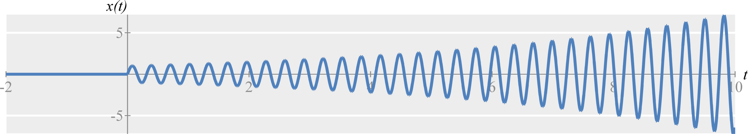
The Fourier Transform and Fourier Series are useful for analyzing a large variety of systems. However, they have` limitations. Specifically, these transforms only exist for energy and power signals. For example, neither the Fourier transform nor Fourier Series exists for $$x(t) = e^{2 t} cos(t) \; .$$ This is because $x(t)$ approaches infinity as $t$ approaches infinity.
However, we if multiply both sides of the equation above by an exponential $e^{-\sigma t}$, $$x(t)e^{-\sigma t} = e^{2 t} cos(t) e^{-\sigma t} = e^{(2 - \sigma) t} cos(t) \; ,$$ the Fourier transform will exist when $\sigma > 2$. When $\sigma > 2$, the signal $x(t)e^{- \sigma t}$ becomes an energy signal. Under this condition ($\sigma > 2$), we can once again use all of the useful properties of the Fourier transform. This is the motivation behind the Laplace transform.
The Bilateral Laplace Transform
The bilateral Laplace transform is defined as $$X(s) = \int_{-\infty}^{\infty} x(t) e^{-s t} dt \; ,$$ where $s$ is a complex number $s = \sigma + j \omega$. The inverse bilateral Laplace transform is defined as $$x(t) = \frac{1}{2 \pi j} \int_{c-j \infty}^{c+j \infty} X(s) e^{s t} ds \; ,$$ where $c$ is a real scalar value within the region of Laplace transform's region of convergence (see below for deals on the region of convergence).
Poles and Zeros
We can represent any Laplace transform representation with the following form: $$X(s) = \frac{\prod_{z=1}^{Z} (s-a_{z}) }{\prod_{p=1}^{P} (s-b_{p})} \; ,$$ where $a_{z}$ and $b_{p}$ are scalar constants for all $1 \leq z \leq Z$ and all $1 \leq p \leq P$. The value $Z$ is the polynomial order of the numerator and the value $P$ is the polynomial order of the denominator. The $a_{z}$ values are the zeros of $X(s)$ (i.e., the values of $s$ such that $X(s) = 0$). The $b_{p}$ values are the poles of $X(s)$ (i.e., the values of $s$ such that $X(s) = \infty$).
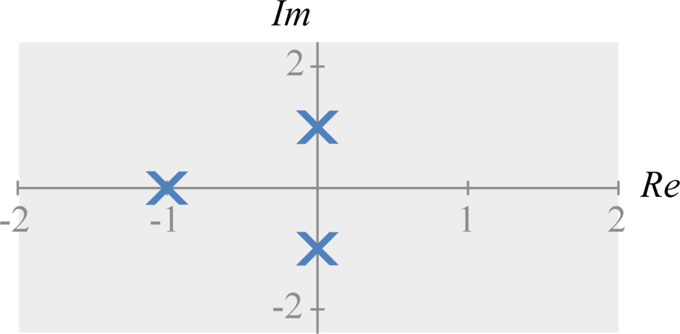
The poles and zeros will be useful for designing control systems and analog filters. The figures below illustrate how we plot poles and zeros in the complex(real-imaginary) plane.

Region of Convergence
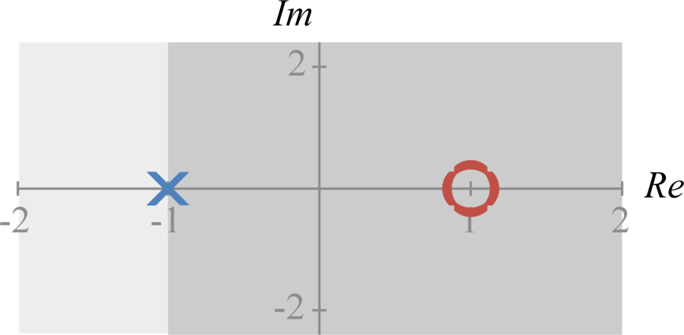
The Fourier transform of $x(t)e^{- \sigma t}$ exists, or converges, for only a specific range of different $\sigma$ values. We refer to this range as the Laplace transform's region of convergence. The region of convergence exists in the complex plane, $\sigma + j \omega$.
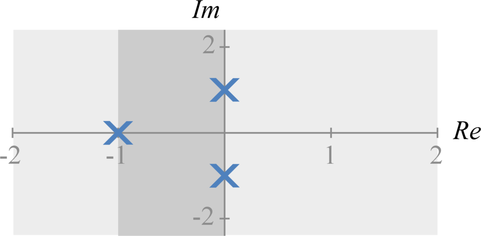
In the complex plane, the region of convergence begins at a pole. If the system is causal, the region of convergence exists for all $\sigma$ and $\omega$ values to the right (larger $\sigma$ values) of the pole. If the system is anti-causal, the region of convergence exists for all $\sigma$ and $\omega$ values to the left (smaller $\sigma$ values) of the pole. If the system has both causal and anti-causal terms, the total region of convergence is the intersection of the region of convergence for each pole.
The Unilateral Laplace Transform
As discussed in the previous subsection, a Laplace representation $X(s)$ can come from many different time-domain signals: the causal signal, anti-causal signal, or a combination of causal and anti-causal signals. The only difference between the Laplace representation of these signals is their regions of convergence. If we assume the time-domain signals are always causal, then there is only one, unique $X(s)$ for any $x(t)$. This is the assumption of the unilateral Laplace Transform.
The unilateral Laplace transform is defined as $$X(s) = \int_{0}^{\infty} x(t) e^{-s t} dt \; .$$ The inverse unilateral Laplace transform is defined as $$x(t) = \frac{1}{2 \pi j} \int_{c-j \infty}^{c+j \infty} F(s) e^{s t} ds \; ,$$ where $c$ is is a real scalar value within the region of Laplace transforms region of convergence. As can be seen, the inverse Laplace transform remains the same as the bilateral transform, but the forward transform is now only valid for causal signals.
Bilateral / Unilateral Laplace transform relationship
The bilateral Laplace transform can be defined as $$\begin{eqnarray*} X(s) &=& \int_{-\infty}^{\infty} x(t) e^{-s t} dt \\ &=& \int_{-\infty}^{0} x(t) e^{-s t} dt + \int_{0}^{\infty} x(t) e^{-s t} dt \\ &=& \int_{0}^{\infty} x(-t) e^{s t} dt + \int_{0}^{\infty} x(t) e^{-s t} dt \; \\ \end{eqnarray*}$$ The first term is the unilateral transform of $x_1(-t) = x(-t) u(t)$ (the anti-causal half of the signal). Note that the Laplace transform of $x_1(-t)$ is $X_1(-s)$ due to the time reversal property. The second term is the unilateral transform of $x_2(t) = x(t) u(t)$. Hence the bilateral Laplace transform is the sum of two unilateral Laplace transforms.
Additional Resources
- From this course
- From Richard Baraniuk's open textbook
- Other online resources