Class 27 (The Z Transform)
Motivation
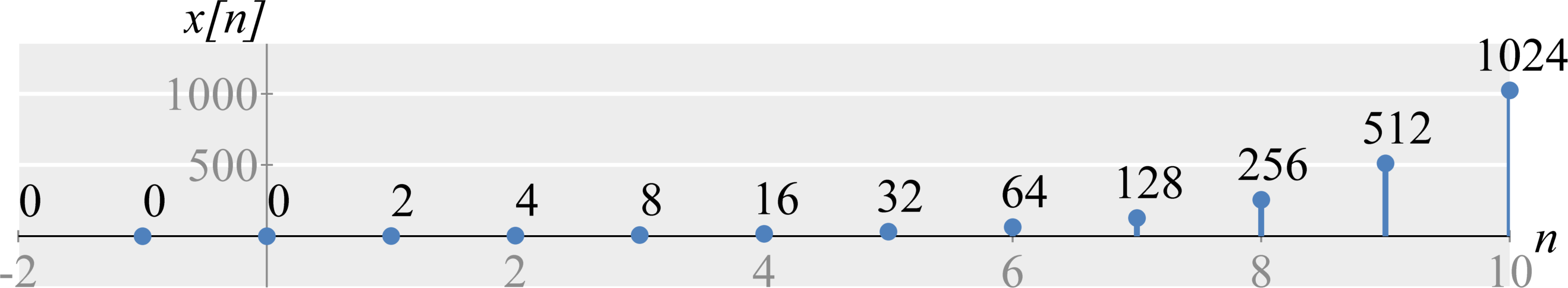
The Discrete-Time Fourier Transform and Discrete-Time Fourier Series are useful for analyzing a large variety of systems. However, they have limitations. Specifically, these transforms only exist for energy and power signals. For example, neither the Discrete-time Fourier transform nor the Discrete-time Fourier Series exists for $$x[n] = (2)^n \; .$$ This is because $x[n]$ approaches infinity as $n$ approaches infinity.
However, we if multiply both sides of the equation above by an exponential $\sigma^{-n}$, we get $$ \sigma^{-n} x[n] = (2 / \sigma)^n \; . $$ the Discrete-Time Fourier transform will exist when $\sigma > 2$. When $\sigma > 2$, the signal $\sigma^{-n} x[n]$ becomes an energy signal. Under this condition ($\sigma > 2$), we can once again use all of the useful properties of the Discrete-Time Fourier transform. This is the motivation behind the Z-transform.
The Bilateral Z-Transform
Definition
The bilateral Z-Transform is defined as $$ X(s) = \sum_{n=-\infty}^{\infty} x[n] z^{-n} \; , $$ where $z$ is a complex number $z = \sigma e^{j \omega}$. The inverse bilateral Laplace transform is defined as $$ x[n] = \frac{1}{2 \pi j} \oint_{\mathcal{C}} X(z) z^{n-1} dz \; , $$ where $\mathcal{C}$ is a closed path around the origin within the region of Z-Transform's transform's region of convergence (see below for deals on the region of convergence).
Poles and Zeros
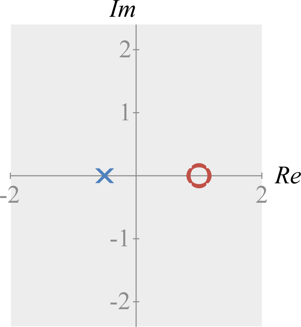
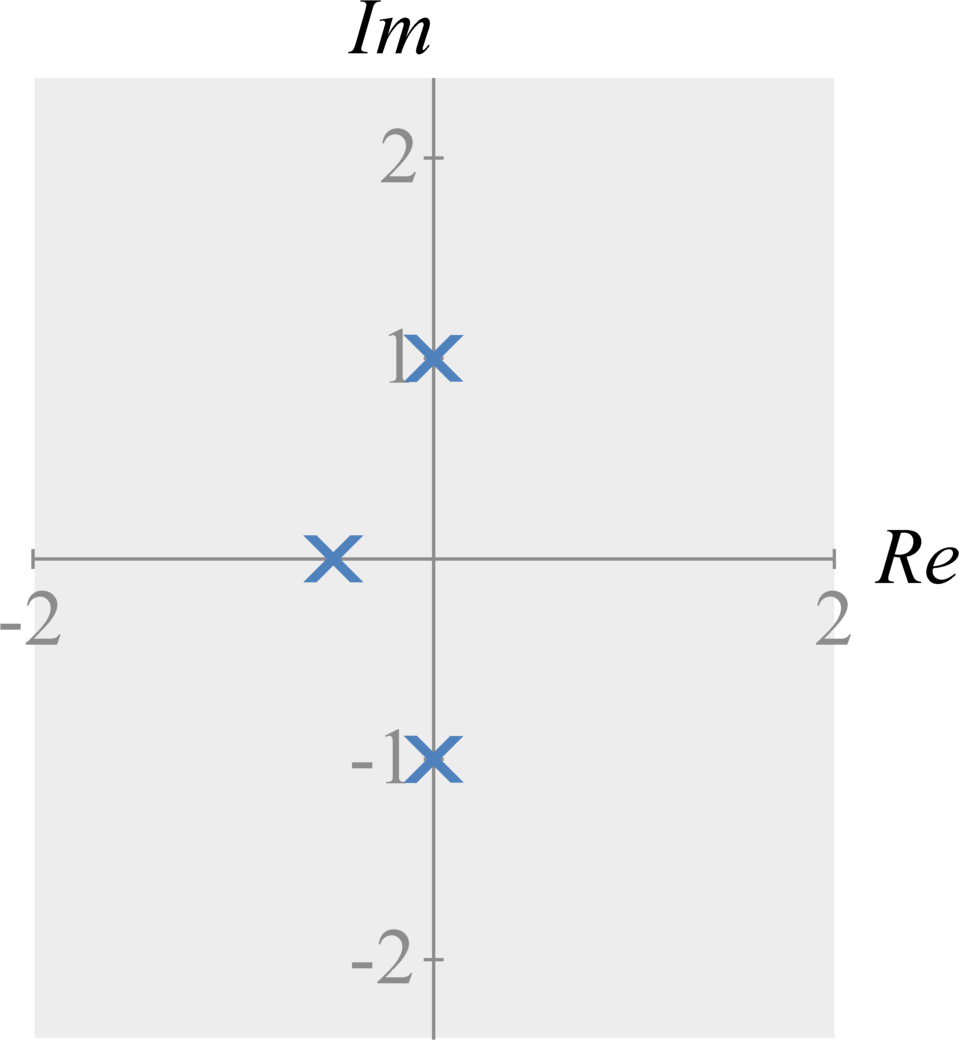
We can represent any Z-transform signal with the following form: $$ \begin{eqnarray} X(z) &=& \frac{\prod_{n=1}^{N} b_{n} z^{-n} }{\prod_{m=1}^{M} a_{m} z^{-m} } \\ &=& \frac{a_0}{b_0} \frac{\prod_{n=1}^{N} \left( 1 -c_{n} z^{-n} \right) }{\prod_{m=1}^{M} \left( 1 - d_{m} z^{-m} \right) } \; , \end{eqnarray} $$ where $c_{n}$ and $d_{m}$ are scalar constants for all $1 \leq n \leq Z$ and all $1 \leq m \leq P$. The value $N$ is the polynomial order of the numerator and the value $M$ is the polynomial order of the denominator. The $c_{n}$ values are the zeros of $X(z)$ (i.e., the values of $z$ such that $X(z) = 0$). The $d_{m}$ values are the poles of $X(z)$ (i.e., the values of $z$ such that $X(z) = \infty$).
The figures below illustrate how we plot poles and zeros in the complex(real-imaginary) plane.
Region of Convergence
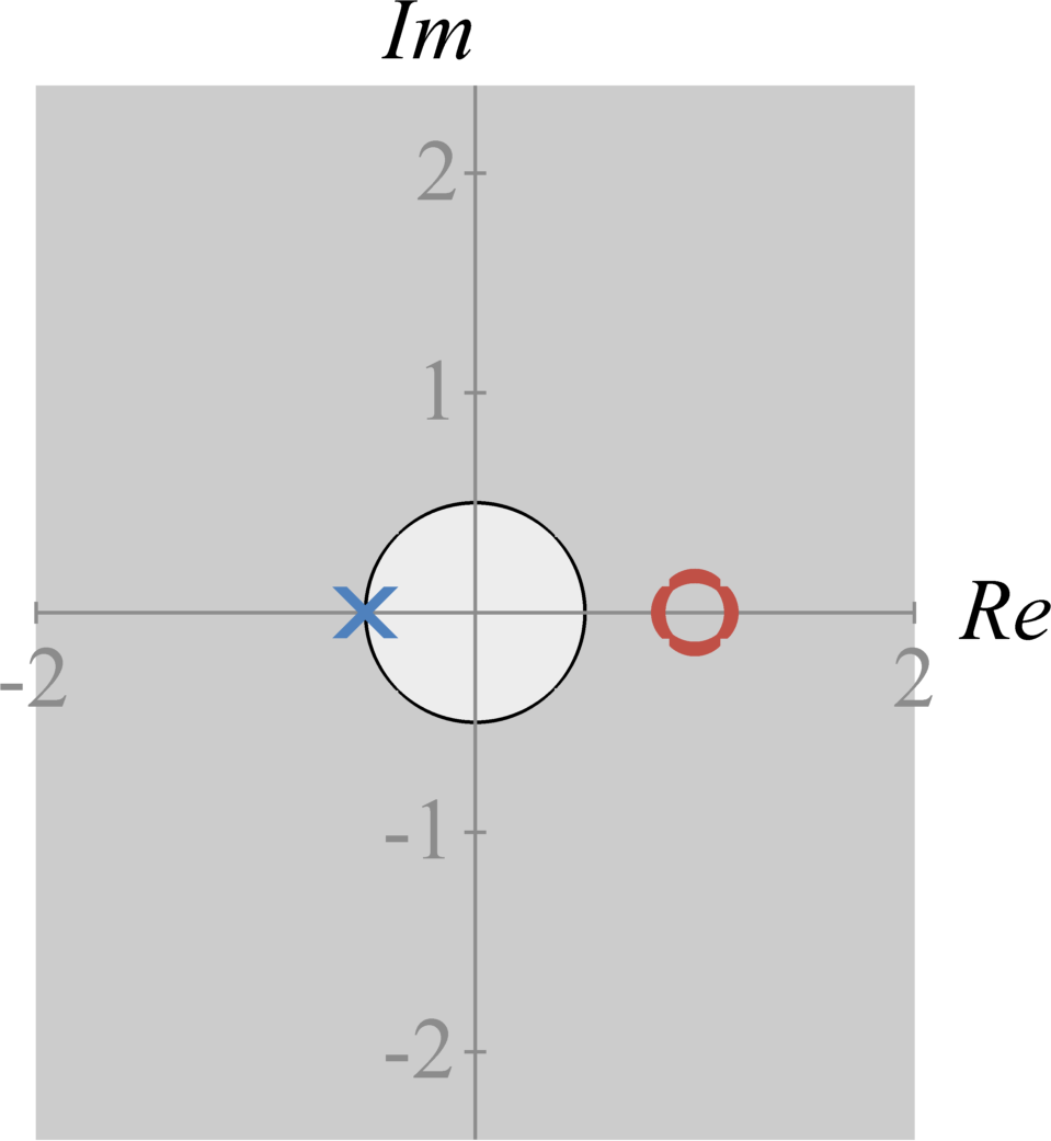
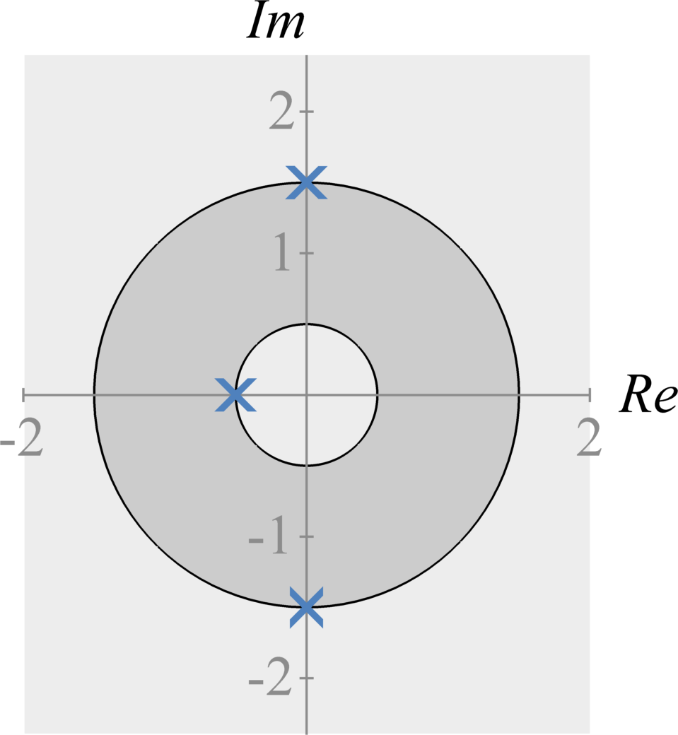
The Discrete-Time Fourier transform of $x[n] \sigma^{-n}$ exists, or converges, for only a specific range of different $\sigma$ values. We refer to this range as the Z-Transform's region of convergence. The region of convergence exists in the complex plane.
In the complex plane, the region of convergence begins at a pole. If the system is causal, the region of convergence exists for all values with a radius greater than $\sigma$ (the real value of the pole) from the origin. If the system is anti-causal, the region of convergence exists for all values with a radius of less than $\sigma$ (the real value of the pole) from the origin. If the system has both causal and anti-causal terms, the total region of convergence is the intersection of the region of convergence for each pole.
Stability
If the pole-zero plot represents the discrete-time transfer function $H(z)$ of a system, then the system is stable when the region of convergence includes the unit circle (circle of radius one). If the region of convergence does not include the unit circle, the system is unstable.
Additional Resources
- From this course
- From Richard Baraniuk's open textbook
- Other online resources