Class 26 (Discrete Fourier Transform Properties)
Circular Convolution
Circular Convolution
When working in the DFT domain, both the time and frequency domains are periodic. Therefore, multiplication in frequency is circular convolution in time. $$ x[n] \circledast h[n] \stackrel{\mathcal{F}}{\longleftrightarrow} X[k] H[k] $$
As with the DTFT, we also observe that multiplication in time is circular convolution in frequency $$ x[n] h[n] \stackrel{\mathcal{F}}{\longleftrightarrow} \frac{1}{N_0} X[k] \circledast H[k] \; ,$$ where $N_0$ is the length of the each signal. The primary difference with the DTFT is that both domains are now discrete.
Periodicity of length $N_0$
In the time domain, circular convolution wraps around the length of the discrete-time signal $N_0$. Therefore, $$x[N+1] = x[1] \; .$$ Or more generally, $$x[n+kN_0] = x[n]$$ for any integer $k$.
As with standard convolution, we can compute circular convolution graphical. We repeat the same steps: we ``time-reverse'' one signal (note that the time reversal is circular too) and shift the signal to the right (circularly). For each shift, we multiply each of the signals and sum the result.
Examples
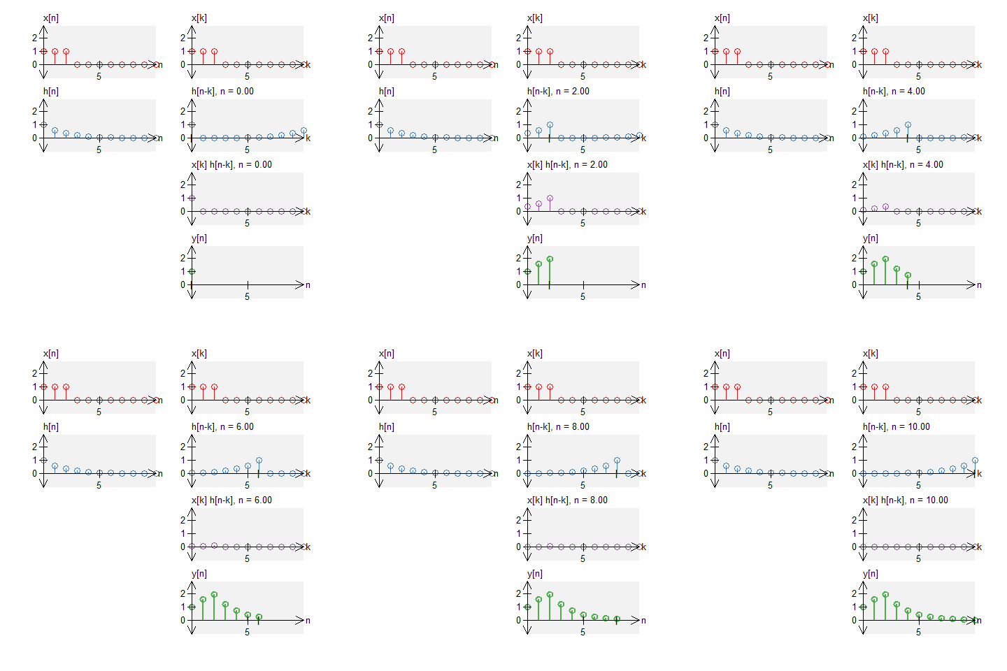
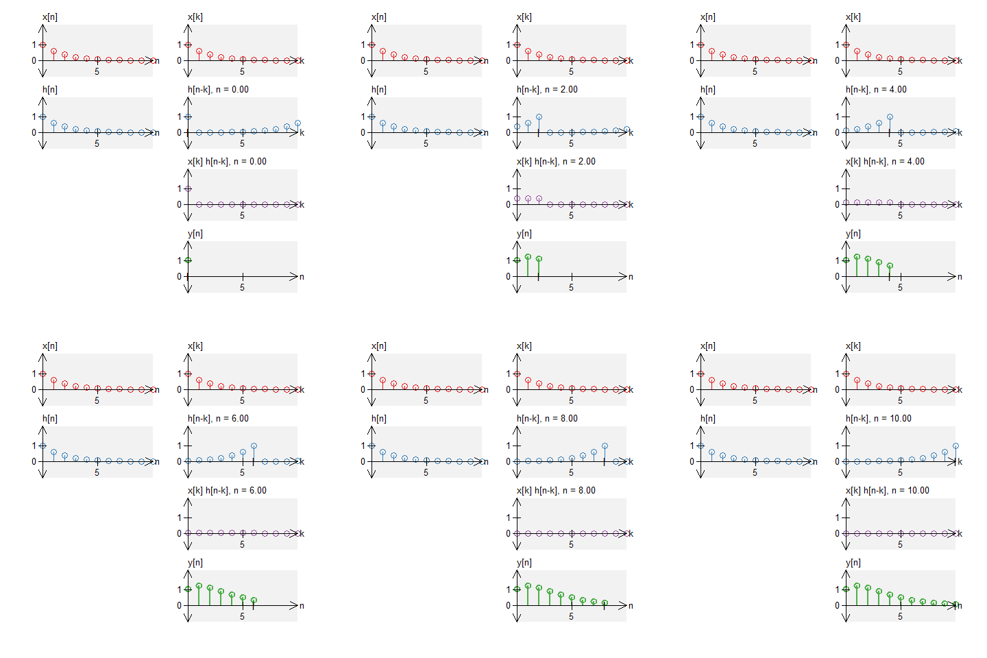
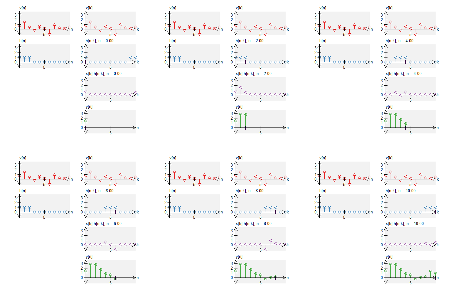
Below are graphical examples of discrete-time circular convolution. We illustrate $y[n] = x[n] \circledast h[n]$, for some input signal $x[n]$ and some system impulse response $h[n]$
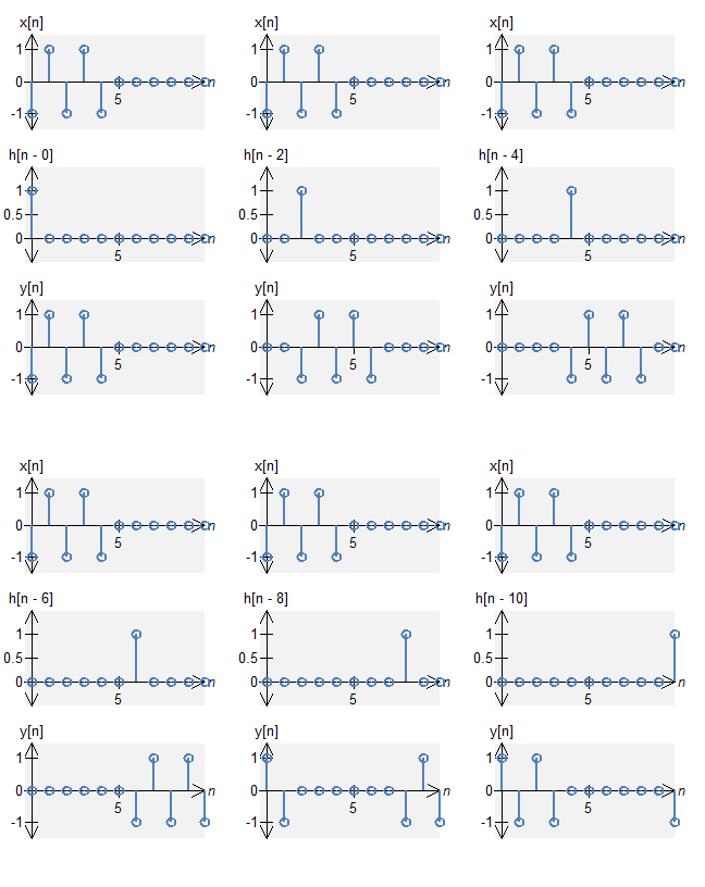
A signal and an impulse at $n=0$
Let a signal $x[n]$ be defined by $$x[n] = -\delta[n] + \delta[n-1] - \delta[n-2] + \delta[n-3] - \delta[n-4] \quad , \quad N_0 = 11 \; .$$ Let $h[n]$ be a length $N_0 = 11$ impulse response defined by $$h[n] = \delta[n] \quad , \quad N_0 = 11 \;. $$ As we would expect from standard convolution, the output of this system would be $$\begin{eqnarray*} y[n] &=& x[n] \circledast \delta[n] = x[n] \\ &=& -\delta[n] + \delta[n-1] - \delta[n-2] + \delta[n-3] - \delta[n-4] \end{eqnarray*}$$

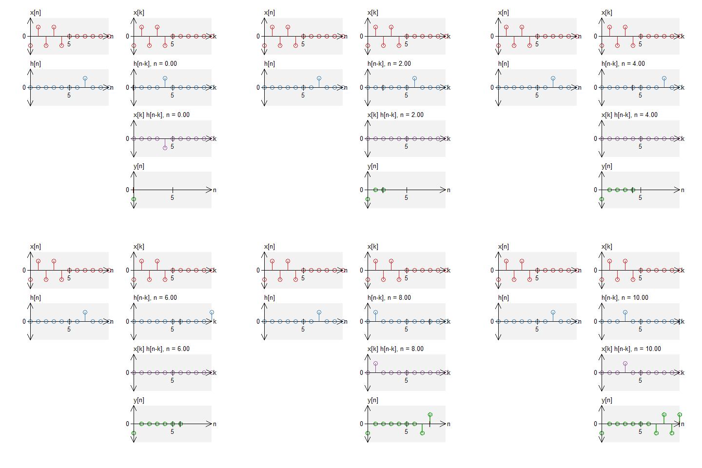
A signal and a shifted impulse
Let a signal $x[n]$ be defined by $$x[n] = -\delta[n] + \delta[n-1] - \delta[n-2] + \delta[n-3] - \delta[n-4] \quad , \quad N_0 = 11 \;, .$$ Let $h[n]$ be an impulse response defined by $$h[n] = \delta[n-7] \quad , \quad N_0 = 11 \;. $$
The circular convolution is defined by $$ \begin{eqnarray*} y[n] &=& x[n] \circledast \delta[n-7] \end{eqnarray*} $$ Now everything is shifting to the right by $7$. However, if the location shifts further than sample $n=10$ (the 11th sample), the value wraps around to $n=0$. Therefore, the results become $$ \begin{eqnarray*} y[n] &=& -\delta[n-\textrm{mod}(7,11)] + \delta[n-\textrm{mod}(1+7,11)] - \delta[n-\textrm{mod}(2+7,11)] \\ && + \delta[n-\textrm{mod}(3+7,11)] - \delta[n-\textrm{mod}(4+7,11)] \\ &=& -\delta[n-7] + \delta[n-8] - \delta[n-9] + \delta[n-10] - \delta[n] \\ \end{eqnarray*} $$ The function $\textrm{mod(} \cdot \textrm{)}$ represents modular division. Notice that the delay of $4+7$ now wraps around to $0$.
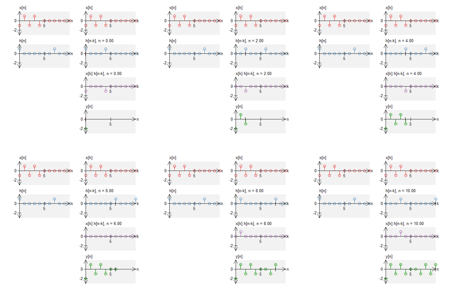
A signal and two impulses
Let a signal $x[n]$ is signal defined by $$ x[n] = -\delta[n] + \delta[n-1] - \delta[n-2] + \delta[n-3] - \delta[n-4] \quad , \quad N_0 = 11 \; . $$ Let $h[n]$ is defined by $$ h[n] = \delta[n] + \delta[n-7] \quad , \quad N_0 = 11 \;. $$
The circular convolution is defined by $$ \begin{eqnarray*} y[n] &=& x[n] \circledast \left( \delta[n] + \delta[n-7] \right) \end{eqnarray*} $$ The result will be the addition of the two results above. Therefore, the results become $$ \begin{eqnarray*} y[n] &=& \left( -\delta[n-7] + \delta[n-8] - \delta[n-9] + \delta[n-10] - \delta[n] \right) + \left( -\delta[n] + \delta[n-1] - \delta[n-2] + \delta[n-3] - \delta[n-4] \right) \\ &=& 2 \delta[n] + \delta[n-1] - \delta[n-2] + \delta[n-3] - \delta[n-4] - \delta[n-7] + \delta[n-8] - \delta[n-9] + \delta[n-10] \end{eqnarray*} $$ Notice that due to the wrap-around effect, we add two value together at $n=0$. This would not happen with standard convolution.
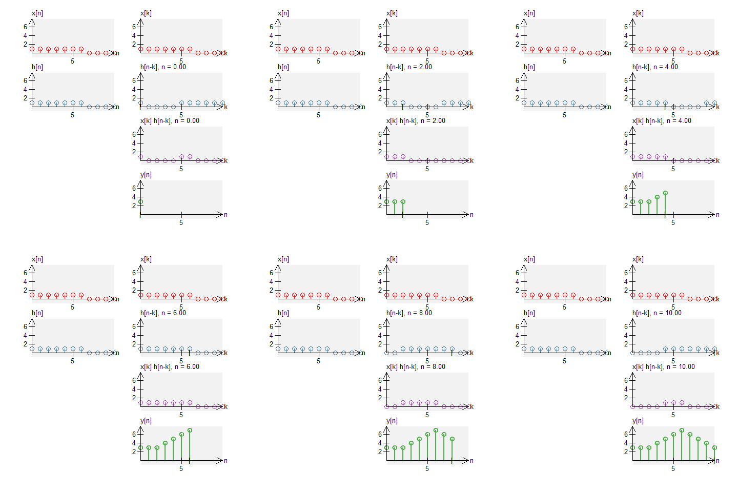
Two long boxes
Let a signal $x[n]$ be a signal defined by $$ x[n] = u[n] - u[n-7] \quad , \quad N_0 = 11 \; . $$ Let $h[n]$ be an impulse response defined by $$ h[n] = u[n] - u[n-7] \quad , \quad N_0 = 11 \;. $$ The circular convolution of these can be graphically shown below. Note that we do not get a triangle (what we would get with standard convolution).
A box and a decay
Two decays
A box and noise
Additional Resources
- From this course
- From Richard Baraniuk's open textbook
- Other online resources