Class 2 (Signals: Their Properties)

Types of signals

Continuous / Discrete

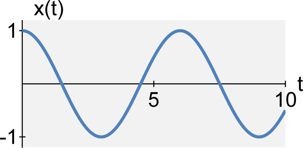
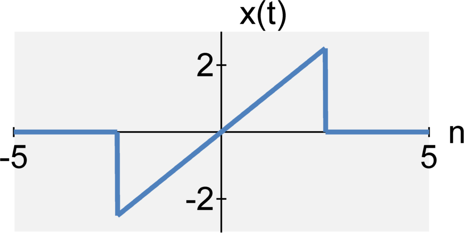
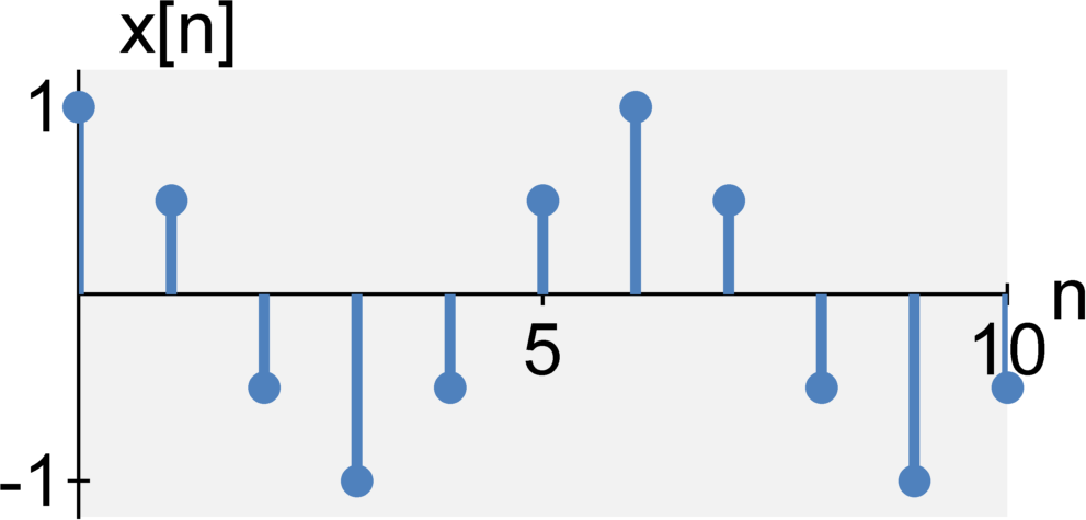
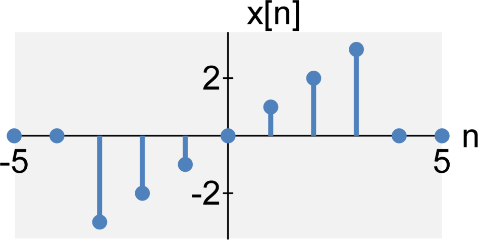
A continuous-time signal $x(t)$ is represented by an uncountably infinite number of dependent variable points (e.g., an uncountably infinite number of values across time).

A discrete-time signal $x[n]$ is represented by an countable (potentially infinite, but not necessarily) number of dependent variable values (e.g., five values across time).

Notation warning: Some texts use the same bracket notation for both continuous-time and discrete-time signals (i.e., $x(t)$ is continuous-time and $x(n)$ is discrete-time). Furthermore, the book denotes discrete-time using $m$ (common in controls literature) rather than $n$ (common in signal processing literature). In this course, we will denote continuous-time signal with round brackets $()$ and discrete-time signals by square brackets $[]$. Further, we will typically use $t$ to denote continuous-time signals and $n$ to denote discrete-time signals. Note though that the dependent variable does not need to be time. It could be anything -- time, space, speed, force, etc.

Analog / Digital

An analog signal x(t) is represented by an uncountably infinite number of independent values (i.e., x) or amplitudes.

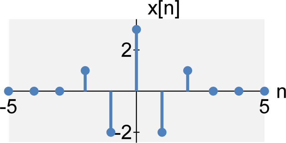
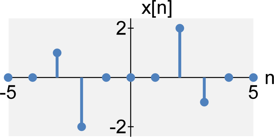
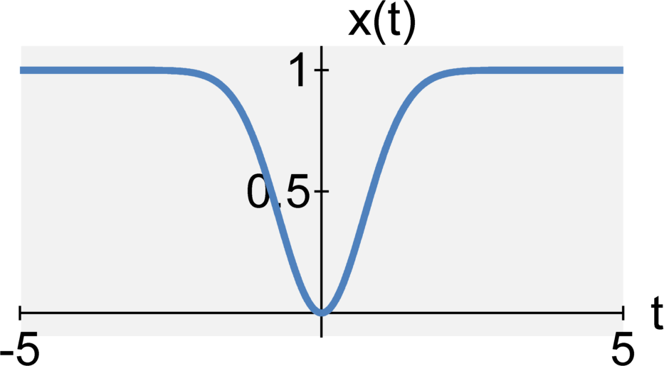
A digital signal x[n] is represented by an countable (potentially infinite, but not necessarily) number of independent values (i.e., x) or amplitudes.

Even / Odd

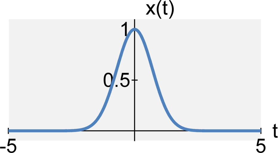
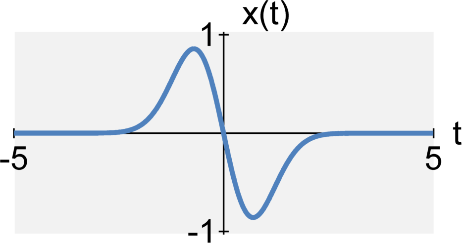
The continuous-time signals $x(t)$ is even when $$x(-t) = x(t)$$ The continuous-time signals $x(t)$ is odd when $$x(-t) = -x(t)$$ The discrete-time signals $x[n]$ is even when $$x[-n] = x[n]$$ The discrete-time signals $x[n]$ is odd when $$x[-n] = -x[n]$$

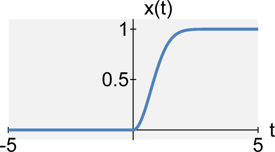
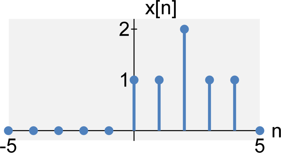
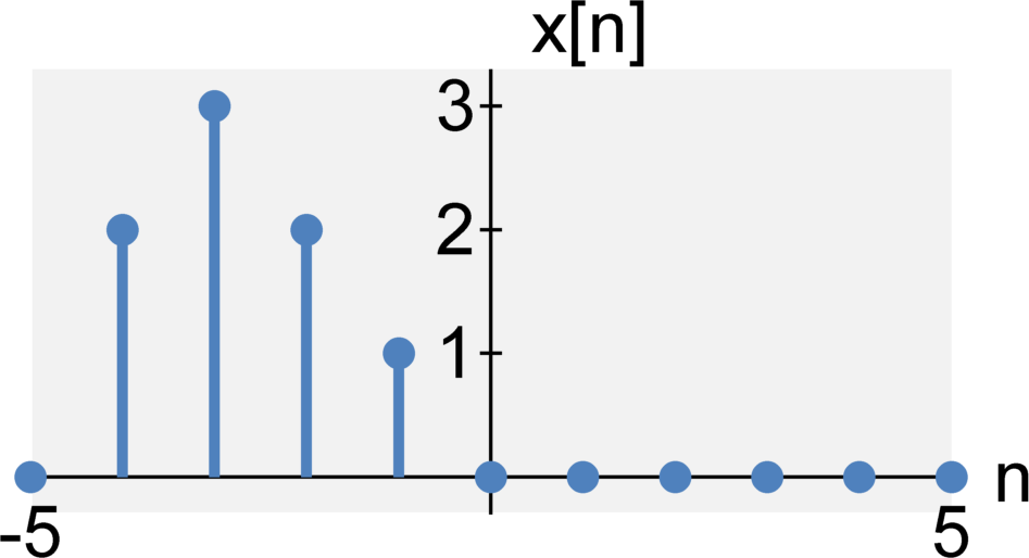
Causal / Acausal

A continuous-time signal x(t) is said to be causal when $$x(t) = 0 \quad \textrm{for} \quad t < 0$$ A continuous-time signal x(t) is said to be anticausal when $$x(t) = 0 \quad \textrm{for} \quad t \geq 0$$ A discrete-time signal x[n] is said to be causal when $$x[n] = 0 \quad \textrm{for} \quad n < 0$$ A discrete-time signal x[n] is said to be anticausal when $$x[n] = 0 \quad \textrm{for} \quad n \geq 0$$ Signals that are not causal are also called acausal. Anticausal signals are are a type acausal signals.

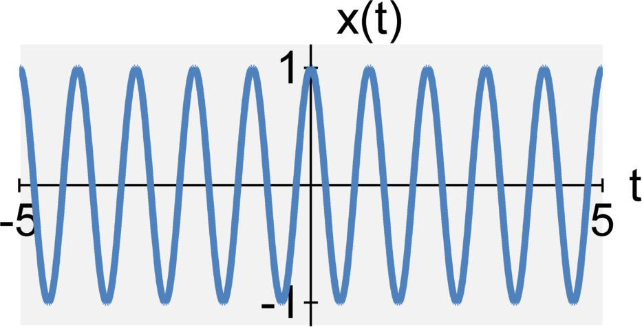
Periodic / Aperiodic

A continuous-time signal $x(t)$ is said to be periodic if some $T_0$ exists such that $$x(t) = x(t+m T_0)$$ where $T_0$ is finite and $m$ can equal any integer value $m = \ldots -2, -1, 0, 1, 2, \ldots$.

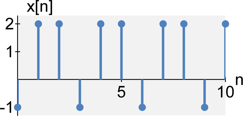
A discrete-time signal $x[n]$ is said to be periodic if some $N_0$ exists such that $$x[n] = x[n+m N_0]$$ where $N_0$ is finite and $m$ can equal any integer value $m = \ldots -2, -1, 0, 1, 2, \ldots$.

Fundamental period/frequency: The smallest $T_0$ or $N_0$ that satisfies the above conditions is known as the fundamental period of the signal. The reciprocal value ($f_0 = 1/T_0$ or $f_0 = 1/N_0$) is known as the fundamental frequency of the signal. We will discuss how to find the fundamental frequency in the next lecture.

Caveat for discrete-time signals: Note that determining periodicity for discrete-time signals is more complicated than it may initially seem. Some signals that are periodic in continuous-time do not satisfy periodicity in discrete-time (for example, $x[n] = \cos(n)$ does not satisfy the periodicity property).

Measures of signal "size"

Energy

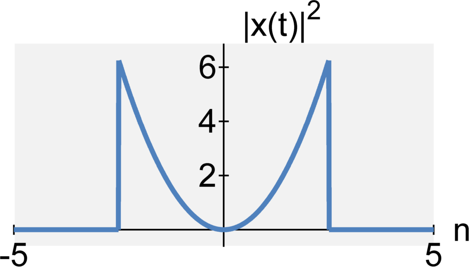
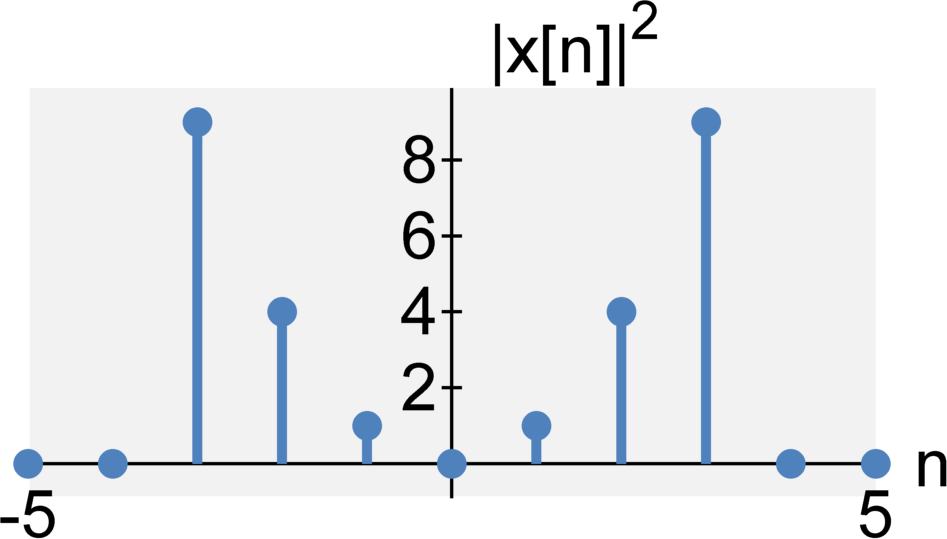
The energy of a continuous-time signal x(t) $$E_x=\int_{-\infty}^{\infty} |x(t)|^2 dt $$ The energy of a discrete-time signal x[n] is $$E_x=\sum_{n=-\infty}^{\infty} |x[n]|^2 $$

An energy signal is a signal with finite energy (i.e., $0 < E_x < \infty$).

Physical Interpretation: Energy, in this context, does not refer to a specific physical property. Instead, it describes the "size" of a signal. Our energy, however, can be related to electrical energy. If $x(t)$ is a voltage signal across a load of resistance $R$, then the energy supplied to that load is $E_x / R$.

Power (sometimes referred to as average power)

The power of a continuous-time signal x(t) $$P_x=\lim_{T \rightarrow \infty} \frac{1}{T} \int_{-T/2}^{T/2} |x(t)|^2 dt \; .$$ When the signal is periodic, the power simplifies to $$P_x=\frac{1}{T} \int_{-T/2}^{T/2} |x(t)|^2 dt \; ,$$ where $T$ is a period of the periodic signal. This is equivalent to saying that the power of a periodic signal is equal to the average energy in one period in the signal.

The power of a discrete-time signal x[n] is $$P_x=\lim_{N \rightarrow \infty} \frac{1}{2N + 1} \sum_{n=-N}^{N} |x[n]|^2 \; .$$ When the signal is periodic, the power simplifies to $$P_x=\frac{1}{N} \sum_{n=0}^{N-1} |x[n]|^2 \; ,$$ where $N$ is a period of the periodic signal. This is equivalent to saying that the power of a periodic signal is equal to the average energy in one period in the signal.

A power signal is a signal with finite power (i.e., $0 < P_x < \infty$).

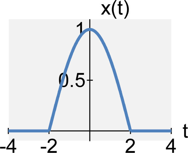
Physical Interpretation: Power, in this context, does not refer to a specific physical property. Instead, it describes the "size" of a periodic signal. Our power, however, can be related to electrical power. If $x(t)$ is a voltage signal across a load of resistance $R$, then the power supplied to that load is $P_x / R$.

Important signal operations

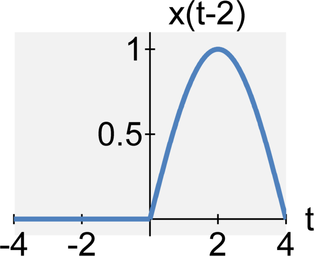
Time shifting

The continuous-time signal $y(t) = x(t-T)$ is the signal $x(t)$ shifted to the right by $T$ units.

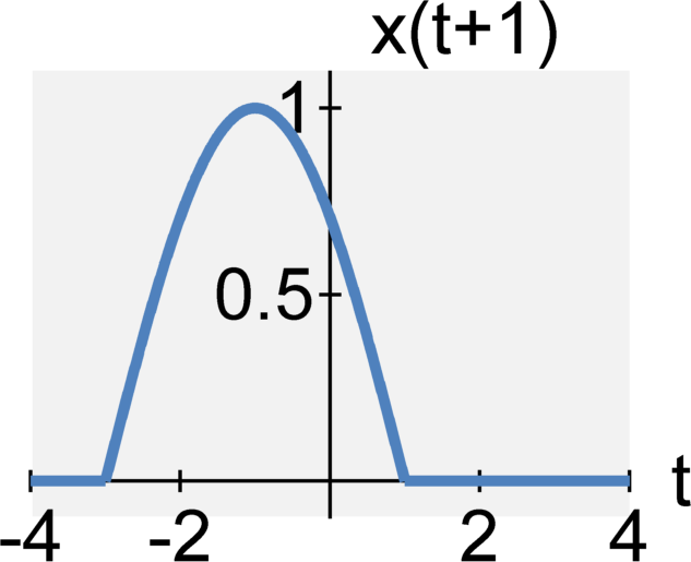
The continuous-time signal $y(t) = x(t+T)$ is the signal $x(t)$ shifted to the left by $T$ units.

The discrete-time signal $y[n] = x[n-N]$ is the signal $x[n]$ shifted to the right by $N$ samples.

The discrete-time signal $y[n] = x[n+N]$ is the signal $x[n]$ shifted to the left by $N$ samples.

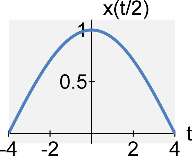
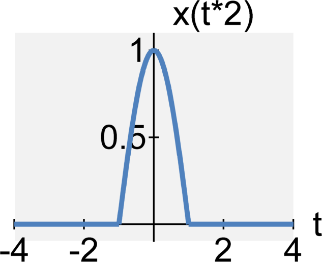
Time scaling

The continuous-time signal $y(t) = x(a t)$ is the signal x(t) condensed by a factor of $a$.

The continuous-time signal $y(t) = x(t / a)$ is the signal x(t) expanded by a factor of $a$.

The discrete-time signal $y[n] = x[a n]$ is the signal x[n] condensed by a factor of $a$.

The discrete-time signal $y[n] = x[n / a]$ is the signal x[n] condensed by a factor of $a$.

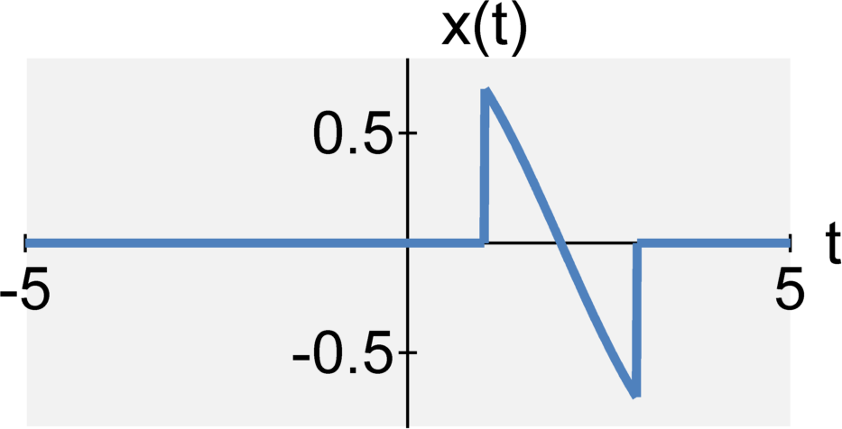
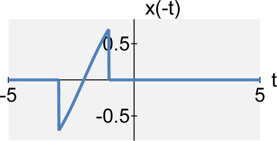
Time reversal

The continuous-time signal $y(t) = x(-t)$ is the time-reversed signal of $x(t)$.

The discrete-time signal $y[n] = x[-n]$ is the time-reversed replica of signal $x[n]$.

Discrete-time Power: From Limit Representation to Periodic Representation

Let $N_0$ be defined as the fundamental period of a periodic signal. Using the assumption that our signal is periodic, the limit representation of discrete-time power can be simplified to $$ \begin{eqnarray} P_x &=& \lim_{N \rightarrow \infty} \frac{1}{2N + 1} \sum_{n=-N}^{N} |x[n]|^2 \\ &=& \lim_{N \rightarrow \infty} \frac{1}{2N + 1} \left[ |x[0]|^2 + \frac{2N}{N_0} \sum_{n=1}^{N_0} |x[n]|^2 \right] \end{eqnarray} $$ We broke up the summation into two terms. The first term is the value of the signal at $n = 0$. The second term is the energy in one period multiplied by $\frac{2N}{N_0}$, which is the ratio of the total range between $-N$ and $N$ (i.e., $2N$) and the fundamental period. That is, for any given $N$, there are $\frac{2N}{N_0}$ periods between $-N$ and $N$. Note that this simplification is not true for any $N$ but is true for the limit of $N$ as it approaches infinity.

To complete our proof, we distribute the $1/(2N+1)$ so that $$ \begin{eqnarray} \lim_{N \rightarrow \infty} \frac{1}{2N + 1} \left[ |x[0]|^2 + \frac{2N}{N_0} \sum_{n=1}^{N_0} |x[n]|^2 \right] &=& \lim_{N \rightarrow \infty} \frac{|x[0]|^2}{2N + 1} + \frac{2N}{N_0(2N+1)} \sum_{n=1}^{N_0} |x[n]|^2 \end{eqnarray} $$ When we evaluate the limit, the first term in the above equation goes to zero as $N$ goes to infinity. The second term, after applying L'Hopsital's rule, converges to $$ \frac{1}{N_0} \sum_{n=1}^{N_0} |x[n]|^2 \; . $$

So, the final solution is $$ \begin{eqnarray} P_x &=& \frac{1}{N_0} \sum_{n=1}^{N_0} |x[n]|^2 \\ &=& \frac{1}{N_0} \sum_{n=0}^{N_0-1} |x[n]|^2 \end{eqnarray}$$

Additional Resources

From this course
- Example problems
- Figure MATLAB code
From Richard Baraniuk's open textbook
Other online resources
- Power and Energy of a signal [from gaussianwaves.com]
- Notation and Basic Signal Properties [from youtube.com]