Class 21 (Aliasing)
Discrete to continuous
Ideal Signal reconstruction
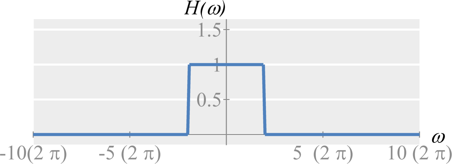
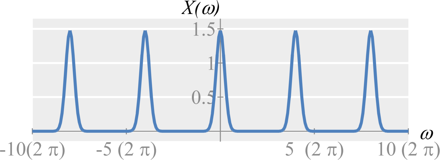
If we satisfy the sampling theorem, we can perfectly reconstruct our original signal with a low-pass filter with a gain of $T_s$. The filter will keep $X(\omega)$ and remove every additional $X(\omega - k\omega_s)$ signal. Generally, the low-pass filter will have cut-off frequency at the half the sampling frequency. Therefore, assuming $\omega_s \geq 2 f_{max}$, $$X(\omega) = \left(\sum_{k=-\infty}^{\infty} \frac{1}{T_s} X(\omega - k \omega_s) \right) H(\omega)$$ where $$H(\omega) = T_s \textrm{rect} \left( \omega / \omega_s \right) \; .$$
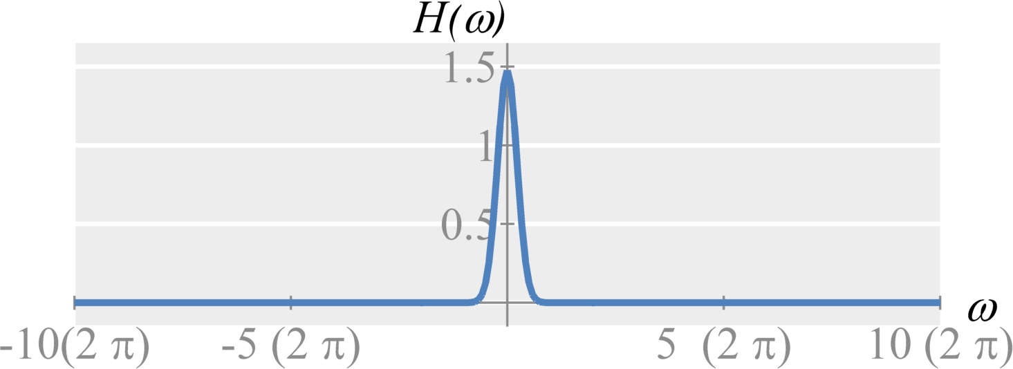
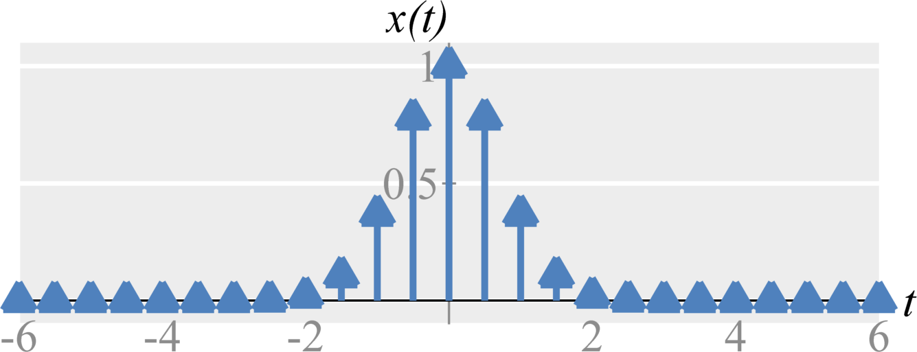
If we apply the convolution property of the Fourier Transform, we see this is equivalent in time to $$x(t) = \left( \sum_{k=-\infty}^{\infty} x(k T_s) \delta(t - k T_s) \right) * h(t)$$ where $$h(t) = \textrm{sinc}\left( ({\omega_s}/{2}) t \right) \; .$$ This tells us that we can convolve (i.e., fit) each sampled impulse with a sinc function to perfectly reconstruct the $x(t)$. This is known as sinc interpolation. Sinc interpolation provides ideal, exact interpolation. Note though that sinc interpolation is difficult to implement in practice.

Aliasing
When we do not satisfy the sampling criteria, we experience aliasing. That is, high frequencies components in $X(\omega)$ are found in the lower frequency range. Aliasing prevents perfect reconstruction and can create strange effects in our signals.
In real-world scenarios, aliasing can be a significant problem. This is because all practical time signals are time-limited. Based on the time-frequency uncertainty principle, this further implies that all practical signals have frequency components from $\omega=-\infty$ to $\omega=\infty$. Therefore sampling any practical signal will result in aliasing.

Anti-aliasing filter
We can prevent, or lessen, the effects of aliasing by removing high frequencies before sampling. We can accomplish this by applying a low-pass filter with cut-off frequency $\omega_s/2$ to the data before sampling. The ideal filter would be defined by $$H(\omega) = \textrm{rect} \left( \omega / \omega_s \right) \; .$$ The anti-aliasing filter removes the data that could contribute to aliasing.
Additional Resources
- From this course
- From Richard Baraniuk's open textbook
- Other online resources