Class 25 (Resampling)
Resampling Discrete-time signals
Overview
Across many situations in signal processing, controls, and communications, we may want to change the rate at which we had originally sampled a discrete-time signal. We refer to this process as resampling. In this lecture, we talk about downsampling (also known as decimation), decreasing the sampling rate by an integer factor $N$, and upsampling (also known as interpolation), increasing the sampling rate by an integer factor $M$.
Downsampling

Downsampling by 2
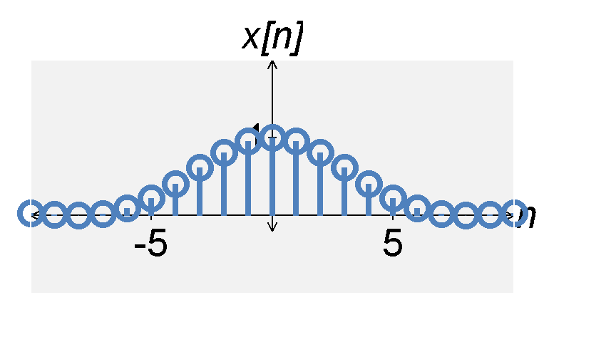
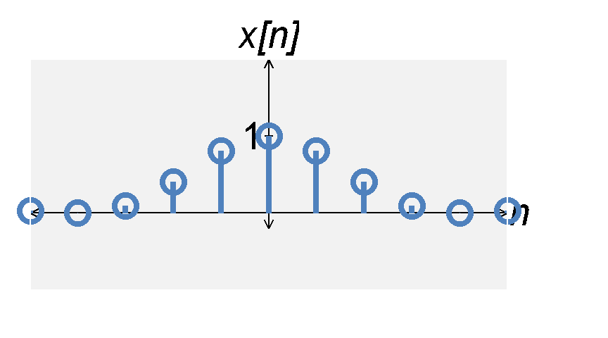
The basic downsampling operation is downsampling by 2. Mathematically, downsampling a signal $x[n]$ by 2 is defined by $$x_d[n] = x[2n] \; .$$ Notice that this is essentially a ``time-shrinking'' of the discrete-time signal by $2$ (and dividing the amplitude by 2). The difference between this operation in discrete-time and continuous-time though is that we must now throw away information. That is, we now only take every other sample.
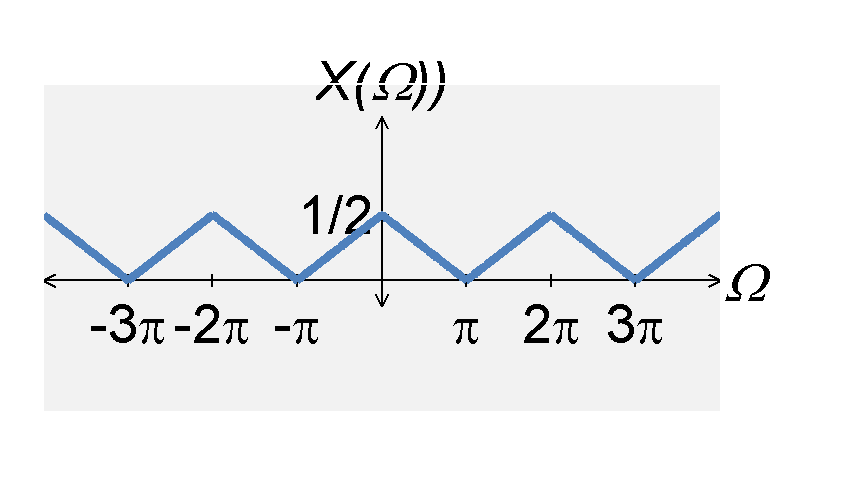
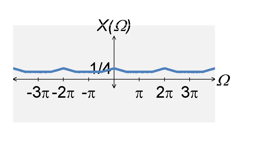
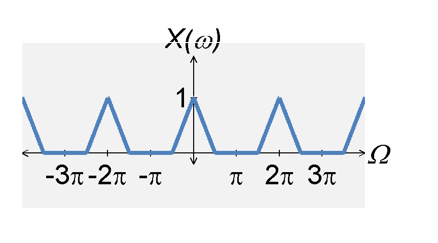
As with continuous-time signals, if we shrink in time, we will stretch in frequency (and devide the amplitude by 2). However, since we work with discrete-time signals, we will ``periodically stretch'' in frequency. That is, we will stretch the frequency content from $-\pi$ to $\pi$ around $\Omega = 0$, we will stretch the frequency content from $\pi$ to $3 \pi$ around $2 \pi$, etc... Therefore, we will stretch each period in the frequency domain signal around the points $2 \pi k$, where $k$ is some integer.
Downsampling by N
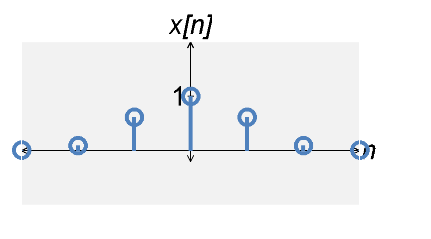
We can extend the concepts above to downsample by any integer number $N$. Downsampling a signal $x[n]$ by $N$ is defined by $$x_d[n] = x[Nn] \; .$$ That is, we keep only every $N$-th sample from $x[n]$. In frequency, we again see the same ``periodic stretching,'' except we now stretch by a factor of $N$ (and we divide the amplitude by $N$).
Aliasing from downsampling
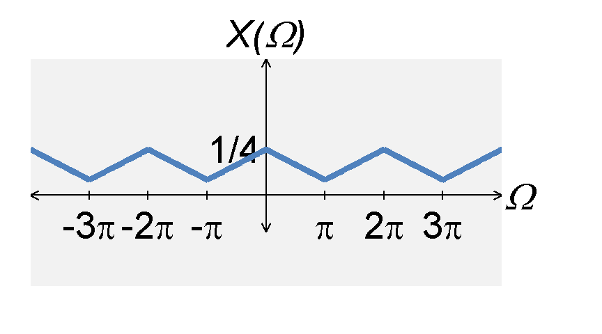
As with regular sampling, we can experience aliasing from downsampling (reducing our sampling rate). Graphically, if the frequency content is stretched too much, we will get overlap (aliasing) and we will no longer be able to perfectly reconstruct the original signal. If the maximum frequecy stretches beyond $\Omega = \pi$, we will get aliasing.
For example, consider a signal $x[n]$ ($X(\Omega)$ in the frequency domain) with a maximum frequency (within the range of $-\pi$ and $\pi$) equal is $3 \pi / 4$. If we downsample $x[n]$ by $2$, the new maximum frequency for the period around $\Omega = 0$ will be $3 \pi / 2$. Similarly the new minimum frequency for the period around $\Omega = 2 \pi$ will be $\pi / 2$. These frequency components will add together, distort the signal, and create aliasing.
Anti-Aliasing
To counter aliasing, signals are often filtered using an low-pass, discrete-time anti-alaising filter before downsampling. To ensure that aliasing does not occur, the cut-off frequency of an ideal filter would have to be $\Omega_c = \pi/N$, where $N$ is the downsampling factor.
Upsampling

Upsampling by 2
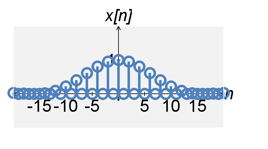
Upsampling is the opposite of downsampling. The basic upsampling operation is upsampling by 2. Mathematically, upsampling is a little more complicated than downsampling, but can be thought of as "stretching" the signal in time (i.e., $x[n/2]$). The difference between this operation in discrete-time and continuous-time though is that by "stretching" the signal, we now have more samples than we have data points.
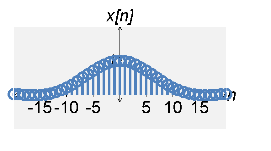
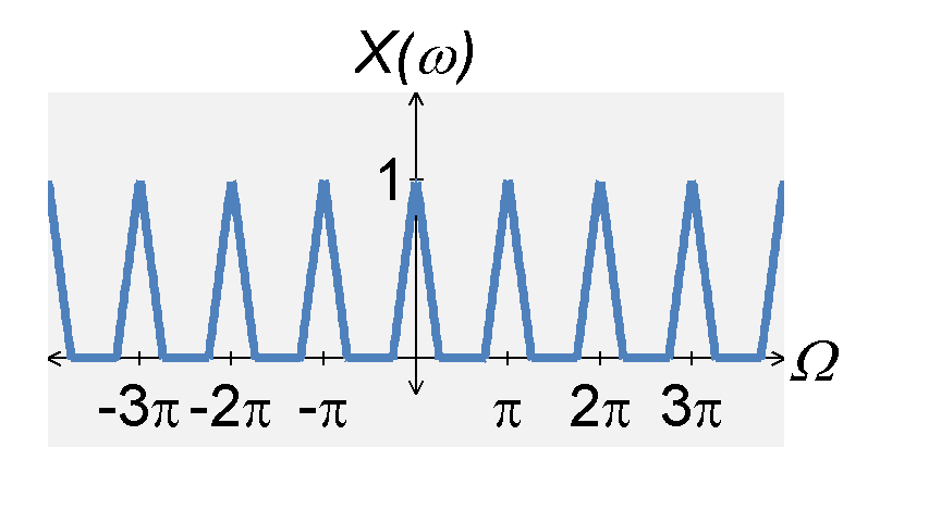
To handle this challenge, we follow two steps. First, we set any new samples to zero. That is, for upsampling by 2, we add one zero between every sample in $x[n]$. This "stretches" the signal in time. As a result, we "shrink" in frequency. However, since we work with discrete-time signals, we will ``periodically shrink'' in frequency. When add a zero between every sample, two things happen.
- First, the periodic frequency domain's period shrinks by a factor of 2. That is, if the DTFT is periodic with a period of $2 \pi$, the upsampled signal will have a period of $\pi$.
- Second, the content in each period frequency-shrinks by a factor of 2.
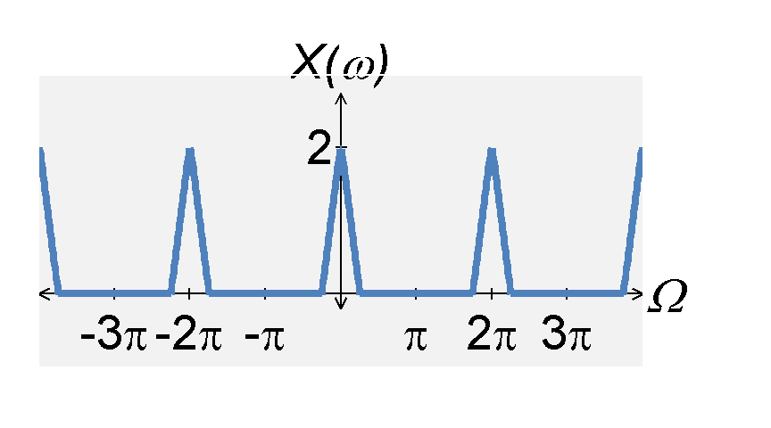
After we add zeroes between every sample in $x[n]$, we apply an discrete-time, ideal low-pass filter with a cut-off of $\pi/2$ and a gain of $2$ to remove frequency content higher than $\Omega=\pi/2$ (within the period between $-\pi$ and $\pi$). In frequency, filtering provides a now shrunken version of the original signal between $\Omega=-\pi$ and $\pi$. In time, filtering determines the values for the zeros that we previously inserted into the signal.
Note that if we now downsampled the result by 2, we would stretch the frequency domain and get the original signal back.
Upsampling by M
We can extend the concepts above to upsample by any integer number $M$. When upsampling a signal $x[n]$ by $M$, we add $M-1$ zeros between each sample. In frequency, we again see the same ``periodic shrinking'' effect, except we now shrink by a factor of $M$. We then apply an ideal low pass filter of with cut-off of $\Omega = \pi/M$ and a gain of $M$. Downsampling the result by $M$ yields the original signal.