Assignment 5
Assignment
In this assignment we will construct a Luneburg lens antenna in the X-band of frequencies. CST has some ability to create objects with spatially varying material properties. In particular there are functions for the Luneburg lens.
Begin by creating a new project (not from a template). Set the units to the usual: mm, GHz and ns. Set the frequency range to the X-band (8-12GHz). Set the background to Normal. Since we will create an antenna in free space, set the Boundary Conditions all to open (add space).
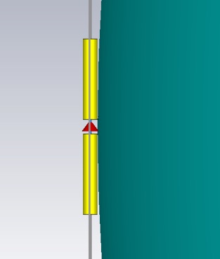
Create a half-wave aluminum dipole antenna with a wire diameter and feed gap both of 1 mm. Create the antenna aligned along the y-axis. (The lens will direct the beam maximum into the z direction). Find the nominal length for an operating frequency at the center of the X-band, then reduce this length by a factor of 0.81. (I found this length tuning factor using the optimizer.)
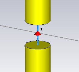
Create a discrete port to drive the antenna.
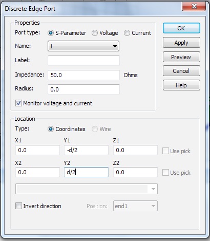
I have used the variable “d” for both the wire diameter and the feed gap. Keep the default Impedance.
Create a farfield monitor and an E-field monitor at the operating frequency. For the E-field monitor use the Subvolume settings to find fields on the y = 0 plane.
Keep the default mesh but increase the accuracy to -50dB and simulate. S11 should have a 20dB dip at the operating frequency.
-
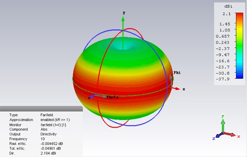
1.Include screen grabs of the S-parameter and the 3D directivity. Make sure you get the efficiencies and the directivity in the screen grab. How does the directivity compare with the usual analytical result for a half-wave dipole?
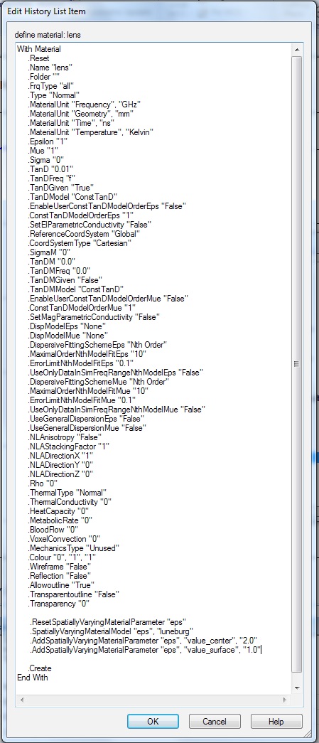
Now create the Luneburg lens. First make a new material. Use Normal Type, vacuum properties.
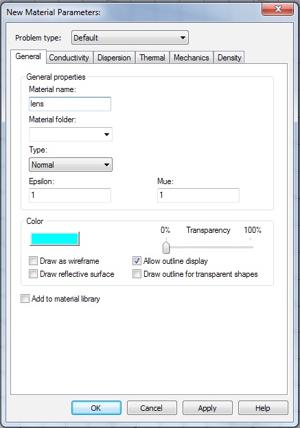
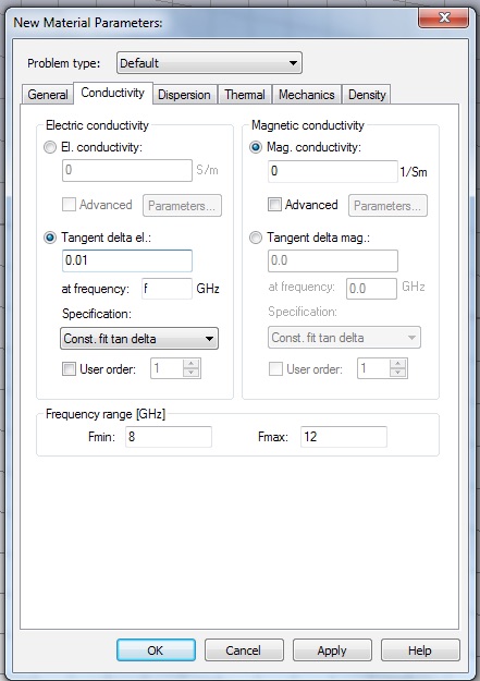
From the Conductivity tab set the Tangent delta el to 0.01, at the operating frequency.
Now open the History List Item for this material and add the following lines
.ResetSpatiallyVaryingMaterialParameter "eps"
.SpatiallyVaryingMaterialModel "eps", "luneburg"
.AddSpatiallyVaryingMaterialParameter "eps", "value_center", "2.0"
.AddSpatiallyVaryingMaterialParameter "eps", "value_surface", "1.0"
to the item, to create the spatially varying material property.
Now create a Sphere to be the lens object. Give the sphere a diameter of 10 λ at the operating frequency, and offset the position of the sphere, so that the sphere is tangent to the dipole antenna.
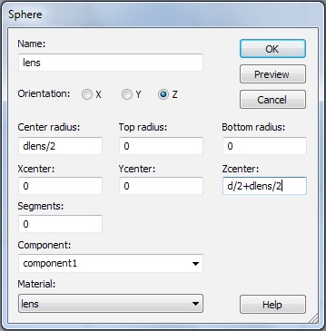
To visualize the sphere as a smooth object you can increase the Triangulation accuracy. This is found here: VIew>>View Options>>Shape Accuracy.
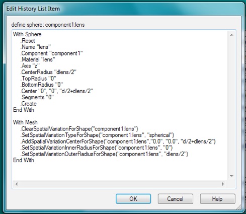
To tell CST to vary use spatial varying material properties for this sphere object, include the following lines. You may need to adjust them to refer to your variable names for the sphere etc.
With Mesh
.ClearSpatialVariationForShape("component1:lens")
.SetSpatialVariationTypeForShape("component1:lens", "spherical")
.AddSpatialVariationCenterForShape("component1:lens","0.0", "0.0", "d/2+dlens/2")
.SetSpatialVariationInnerRadiusForShape("component1:lens", "0")
.SetSpatialVariationOuterRadiusForShape("component1:lens", "dlens/2")
End With
You can add the lines after the Sphere definition.
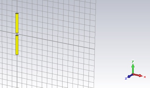
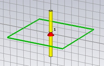
Add any symmetry planes that are compatible with your structure and source excitation. The simulation runs twice as fast for each symmetry plane you add.
2. Provide a screen grab of the symmetry planes. Explain why you chose these planes (both their orientation and type.)
Open and reset the E-field monitor, so that the plane extends all the way through the simulation domain.
The dipole resonance gets shifted by the presence of the lens. Reduce the length of the dipole from 0.81 to 0.77 of the nominal λ/2 length to keep the resonance at the operating frequency.
Simulate.
-
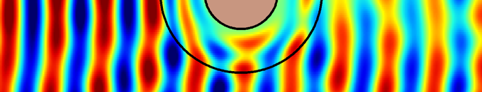
3.Include screen grabs of the S-parameter, the local electric field, and the 3D directivity. For the local E-field (on the y=0 plane), plot the y-component and adjust the scale so that the action of the lens on the wavefronts can be observed. Make sure you get the efficiencies and the directivity in the 3D directivity screen grab.
-
4.Does the directivity agree with the result for an ideal (i.e. uniform) aperture of the same area? Suggest some reasons for any difference.