Assignment

There are at least two different ways to characterize a material with electromagnetic simulation software: S-Parameter simulation and Eigenmode solution.

S-Parameters

In this assignment, we will find the S-parameters of a slab of Teflon by performing a time domain simulation. We will find these S-parameters with the default phase reference (incorrect) and with the phase reference de-embedded to the Teflon-vacuum interface (correct). Then we will compare the simulation results with an analytical formula.

Launch CST Studio Suite (from the desktop.) Accept the university version agreement.

Open CST Microwave Studio, the icon in the lower left corner.

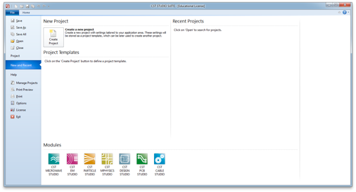
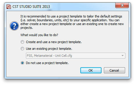
Then select Do no use a project template and click OK.

Let’s set up a few basic things, before we do any modeling.

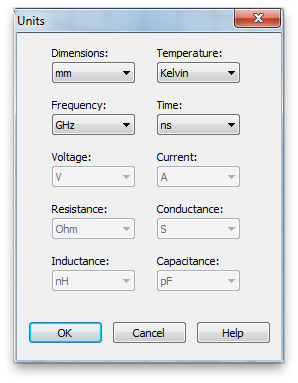
Click the Home tab, then click Units on the command ribbon. Set the units to mm, GHz and ns (nano-seconds). These will be most convenient units for the scale we will be working at.

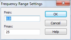
Next select the Simulation tab, and click Frequency.  Set the maximum frequency to 25 GHz.

Click Background. Set the background material to Normal, instead of PEC. The values for the background Epsilon and Mue can be adjusted using the Properties... button, but just leave these values at unity. These are the material properties relative to vacuum. So we are setting the background material to vacuum. (Note that the properties of air are very close to vacuum.)

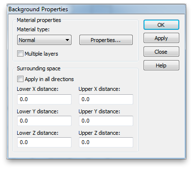
It’s a common mistake to omit this step and not realize that all the undefined regions in your simulation are the default, PEC, that is a perfect electric conductor.

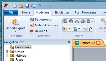
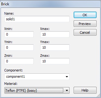
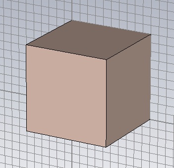
Now select the Modeling tab. Use the Brick tool to create a cube of Teflon, 10mm on side. The tool is a small cube on the command ribbon.

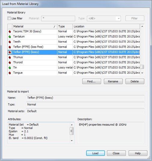
Hit escape to pull up the numerical entry panel. Set the dimensions as shown and select [Load from Material Library...] from the Material: menu. Load the lossy Teflon from the material library as shown.

The Teflon cube.

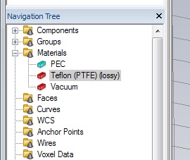
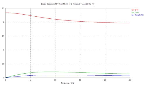
Let’s increase the lossiness of the Teflon to make the simulation results a bit more interesting. Double click the Teflon material in the Materials folder of the Navigation Tree.

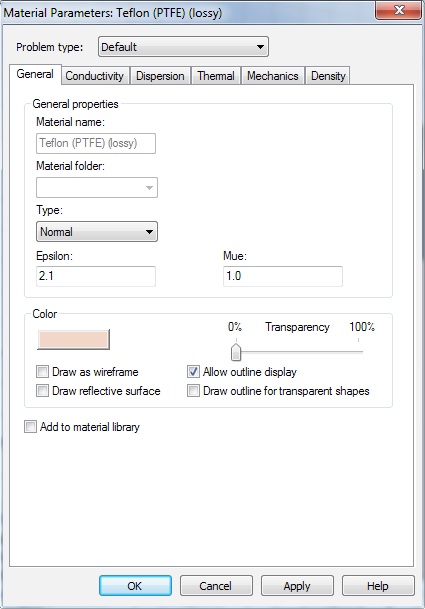
Select the Conductivity tab, and increase the tanδ by a factor of  500, to 0.1.

The resulting changed material properties versus frequency will be shown.

You can return to the 3D cad layout by clicking the 3D tab below the display window.

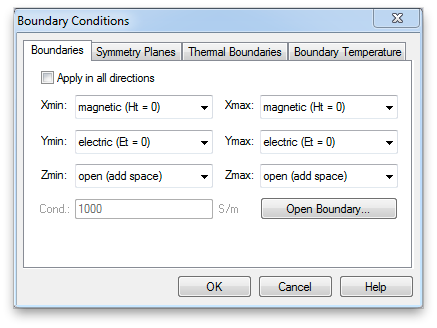
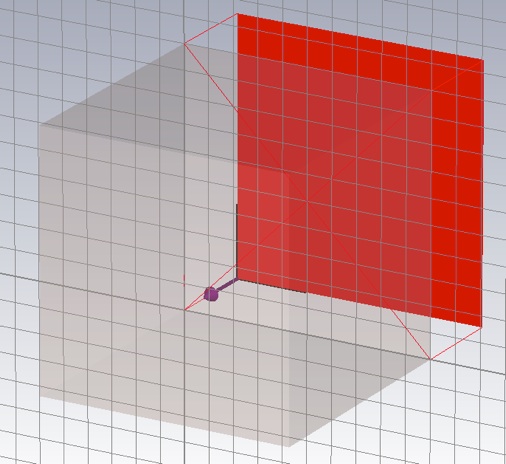
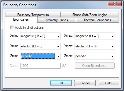
Next go back to the Simulation tab, and click Boundaries. Set the boundary conditions to magnetic (Ht=0) on the two X-planes, electric (Et=0) on the two Y-planes and open (add space) on the two Z-planes. This creates a TEM waveguide, something difficult to do in the lab, but easy in simulation.

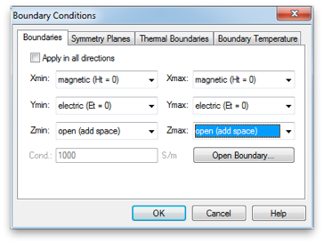
If you re-open the Boundaries panel, all the set boundaries will show color coded as follows.

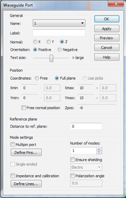
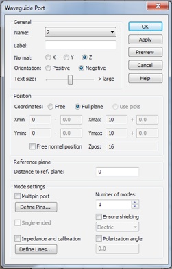
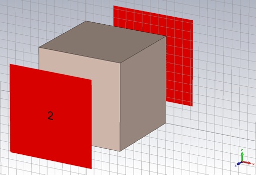
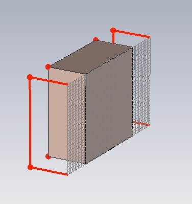
By clicking Waveguide Port, create two waveguide ports. Use all default values, except choose Negative orientation for the second one.

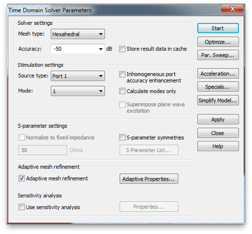
Now click Start Simulation, which will open the Time Domain Solver by default. (You can select other solvers on the Home tab.) Set the Accuracy to -50 dB, the Source Type to Port 1 and check the Adaptive mesh refinement box. Start the simulation.

Click Mesh View, so you can watch the adaptive mesh refinement as it proceeds.  As the mesh refinement proceeds, try different mesh view options to visualize the 3D structure of the mesh. Note that at the beginning of each simulation, the ports are adaptively meshed before the volume is simulated.

Port 2 mesh.

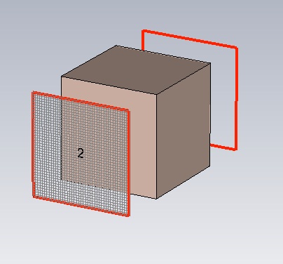
Simulation domain volumetric mesh, Normal: X-plane shown.

You can also watch the convergence by viewing: 1D Results>>Adaptive Meshing>>S-Parameters>>S21 or S11 from the Navigation Tree, on the left. The default view is the real part of the S-Parameter.

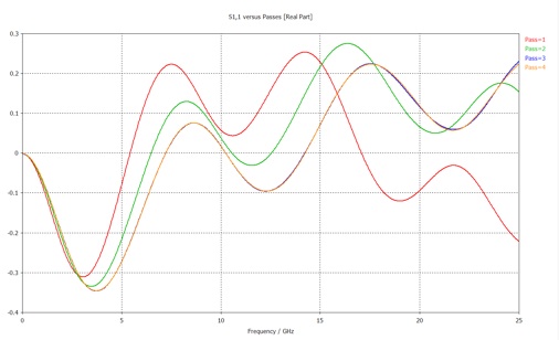
The simulation stops when the S-parameters converge. You will be asked if you want to disable further adaptive meshing. Click yes.

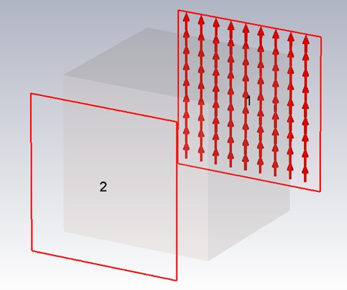
The S-parameters represent the amplitude and phase of the reflected and transmitted waves relative to the incident wave. The waves in question are the modes of the ports. It is very important to always look at the port modes to see if they are as you think.

From the Navigation Tree select 2D/3D Results>>Port Modes>>Port 1>>e1. (Also look at h1 as well as Port 2.)

Now we want to export the magnitude and phase of just the final S-parameters (not all the adaptive passes). Click 1D Results>>S-Parameters. Then click Polar in the 1D Plot tab.

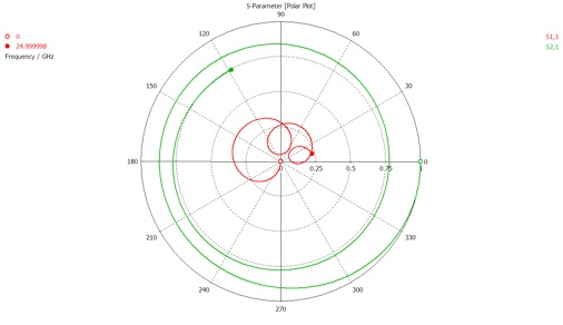
Select the Post Processing tab, and click Import/Export. Then select Plot Data (ASCII)... and save the text file to an appropriate location. The file should look like this:

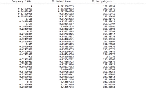
Load the data into your favorite analysis package (e.g. MATLAB or Mathematica). Plot the linear magnitude of S11 and S21 (second column of file) versus frequency (first column of file). (Note that the S11 data is at the top of the file and the S21 data begins half way down.) Make sure this plot looks like the S-parameter plot in Microwave Studio that you get when you select Linear from the 1D Plot tab.

You will also need the material properties for Teflon that were used in the simulation. In the Navigation Tree select 1D Results>>Materials>>Teflon (PTFE) (lossy)>>Dispersive. Again, select the Post Processing tab, and click Import/Export. Then select Plot Data (ASCII)... and save the text file to an appropriate location.

The resulting file will contain the real and imaginary parts of the Teflon permittivity, and the their ratio, tanδ. Note, that CST uses the engineers’ convention for the time dependence of harmonic functions

and not the physicists’ convention

so that, for example, passive materials have a negative imaginary part. However, CST uses the primed and double primed symbols to represent the real and negative imaginary part of a complex quantity

Also, tanδ is usually considered to be a positive quantity for passive materials, regardless of convention.

tanδ is a commonly specified material property that gives a measure of the lossiness of a material.

1. 1.Now plot the corresponding analytical result for the S-parameters using equation 1 and 2 of this article and the material properties for Teflon that you exported from CST. For each S-parameter, put the curves for the simulation and analytical results in the same graph for comparison. Adjust the styles and/or point density so both results can be clearly seen.
   

Note that this is a physics article so that coefficients r and t’ are related to S11 and S21 through the complex conjugate

The wave vector, k, in equation 1 and 2 is the free space value and the speed of light in the units we are using is about 300.

Also, d, is the thickness of the material, which is in our case 10mm. The refractive index, n, and the relative impedance, z, are related to the relative permittivity, ε, and the relative permeability, μ, in the usual way

Now lets see if the simulation and analytical results agree in phase as well as magnitude.

2. What is the significance of the frequencies at which S11 is a minimum? (Hint: consider the phase advance that a wave undergoes making a round trip inside the Teflon slab.) Do these frequencies agree with the simple formula that describes the condition? (You can use the nominal value of 2.1 for the permittivity of the medium for calculating the wavelength or propagation constant.)

3. On one graph plot the real and imaginary parts of S11 versus frequency, both from simulation and equation 1 and 2. (Make sure you conjugate either the simulation or analytical results so that both use the same time harmonic function convention.) Make a second graph of this type for S21.

4. Explain why these results do not show agreement between simulation and analytical results.

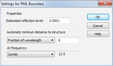
Now we will fix the problem by de-embedding the simulation S-parameters. We will accomplish this by shifting the port reference planes. The open (add space) boundary assignment has added some background media of thickness equal to one eighth of the wavelength (in the background medium) at the center frequency (12.5 GHz). You can check or change these settings by clicking the Open Boundary... button in the Boundary Conditions panel.

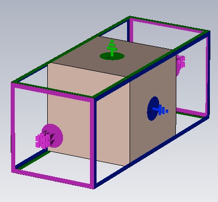
Now open the Waveguide Port panel by double clicking a port in the Navigation Tree.

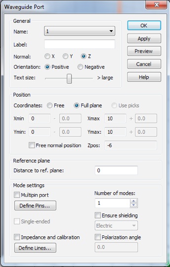
Enter the correct value in the Distance to ref. plane box. (You may enter an expression that uses arithmetic operators if you like.) A negative value moves the reference plane in toward the Teflon block. Make sure the reference plane lies on the block as shown.

Do the same for the other port, then re-run the simulation and export the data. (The current mesh is fine. You don’t need to re-run the adaptive meshing, so keep that box unchecked.)

5. Re-do the graphs, as in 2 above, with the new data. How is the agreement now?

Eigenmode Solution

From the Eigenmode Solver we can obtain the dispersion relation, that is the functional relationship between the frequency, ω, and the propagation constant, β. This relationship conveys a lot of information, particularly the phase (and group) velocity, and thus the refractive index.

The Eigenmode Solver, can find this relationship for multiple bands, but we will look at just the lowest band. Lossy (i.e. complex) and dispersive (i.e. frequency dependent) material properties significantly slow computation and complicate the results, so we will use the default solver settings which ignore such properties. The Teflon will be modeled as a material with a constant, real-valued, permittivity, of 2.1.

We  won’t need the waveguide ports, in fact, they will cause an error, so we well delete them. In the Navigation Tree, right click each port, to bring up the context menu, and select delete.

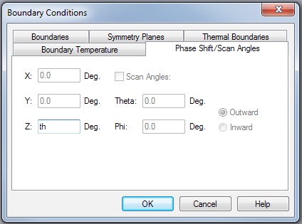
We wish to find frequencies for a range of values of the propagation constant. The way one specifies the propagation constant is by using periodic boundary conditions with a Phase Shift. Change the boundary conditions on the faces that used to have the ports to Periodic.

Then select the Phase Shift/Scan Angles tab and put in a variable for the Z phase shift. (I used th.) Click OK and supply an initial value when prompted. Zero is fine.

Now, change the Solver type to Eigenmode. You can do this from the drop down menu on the Home tab.

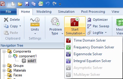
Open the Eigenmode Solver Parameters panel by clicking Start Simulation.

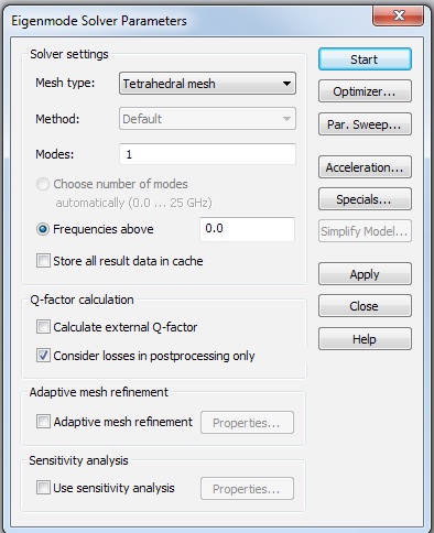
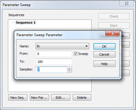
We will leave all of these parameters at their default values, but we do need to set up a Parameter Sweep, to simulate a range of different values for the propagation constant. Click the Par. Sweep… button.

In the Parameter Sweep panel, click New Seq. and then New Par… . Choose the parameter you created from the Name: menu, and specify 7 samples from 0 to 180 degrees, i.e. 30 degree steps.

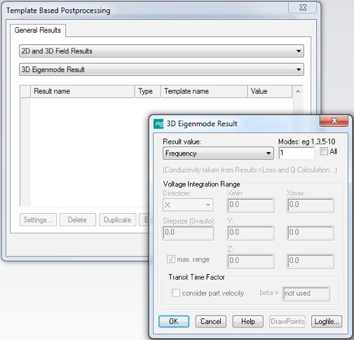
Since the system will run multiple simulations, it does not, by default, save any results. To specify what is saved after each simulation, click Result Template… .

From the top menu, select 2D and 3D Field Results, and then from the bottom menu select 3D Eigenmode Result. The default setup parameters in this panel will save one eigenmode frequency, which is exactly what we want. Click OK.

Now close the Template Based Postprocessing panel to return to the Parameter Sweep panel. Click Start to run the seven simulations.

When the simulations are complete, find and select the Frequency (Mode 1) item in the Tables folder of the Navigation Tree. Export this data as before.

6. 6.Plot a dispersion diagram (ω vs β) with the data points from the simulation and a theoretical curve for Teflon. Note that the material properties used for the Eigensolver are non-lossy, non-dispersive properties. How well do the simulation data points and the theory curve agree?
   

7. Does the dispersion diagram contain information about the refractive index and/or the impedance?