Assignment

We will simulate something vaguely resembling the iPhone 4 antennas and determine their properties with and without a finger on the, so called, death spot.

First construct a model that captures the basic configuration of the handsets antennas. It is possible that (as this person believes) the antennas are essentially slot antennas as outlined in an Apple patent.

Use our usual units (mm, GHz, nS). Set the frequency range to 0 to 3 GHz. Set the Background Material to Normal with Epsilon = Mue = 1.

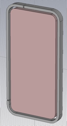
The innards (between the glass front and back) can be modeled as a single brick of metal. The outer-most part will be a steel band circumscribing the handset with two splits to separate the GSM antenna from the WiFi/GPS/Bluetooth antenna. Use Copper (annealed) (lossy) for the innards and Steel-1010 (lossy) for the outer band, though obviously these are rough approximations. Use global parameters for all the geometric properties so we will have ample tuning capability. Use blend radii that lead to uniform cross-sections in the outer band and the slot.

Use global parameters and formulas to specify the geometry. For example:

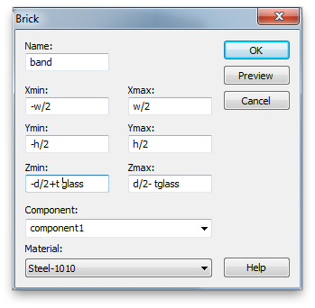
For initial values use:

exterior corner radius = 10mm

lateral exterior dimensions use Apple tech specs

metal thickness = 6.3 mm

glass thickness = 1.5 mm

outer band width = 2.5 mm

slot width = 2 mm

left lower slit position, below center = 43 mm

left upper slit position, left of center = 10 mm

split width = 1 mm

Now add the glass to the front and back. Use Glass (Pyrex) (lossy) because we do not have a model for the fancy aluminosilcate glass that Mr. Jobs specified.

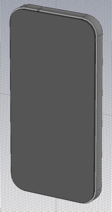
Set the glass back from the edge as on the real handset. For an initial value of the set back use 1 mm, and again, use blending radii such that all blends have the same center of curvature.

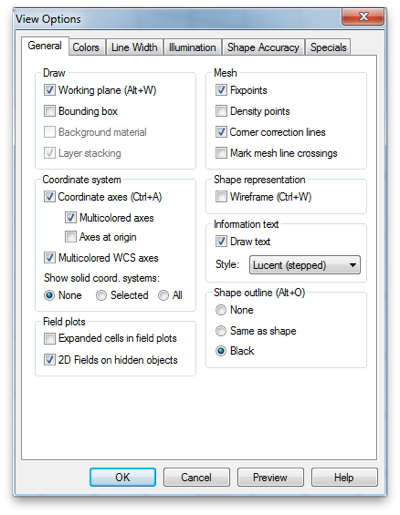
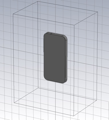
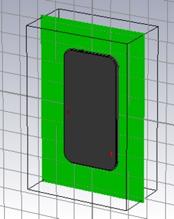
Set all boundaries to open (add space), since we want the antennas to radiate into an infinite space and we will not need to de-embed any waveguide ports. You may want to see where the simulation domain Bounding Box is. You can set this to be visible in the View Options panel accessible from the View Tab.

Now add the discrete ports that will function as antenna feeds. Use the default 50 Ohms for the impedance (a guess) and check the Monitor voltage and current box. The Discrete Edge Port panel is accessible from the Simulation Tab.

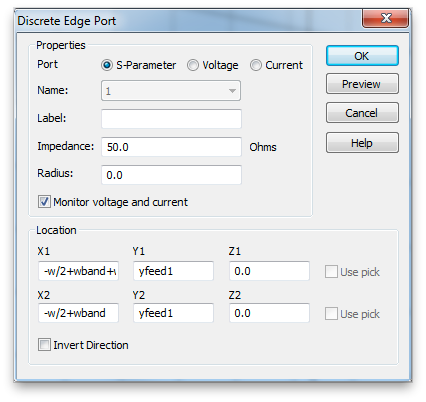
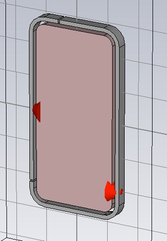
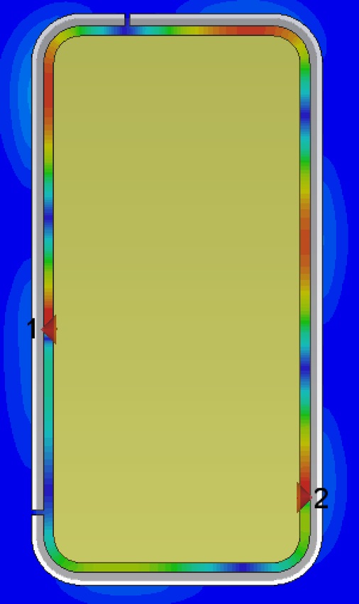
When selected the port is shown as a blue line with a red cone indicating the polarity. It should span the slot, and should probably lie in the center (front to back) of the slot. Use the handset center as the initial value of the vertical position. You probably want to zoom in and hide the glass to confirm the port is where it ought to be.

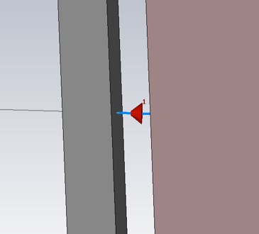
Add another discrete port for the other (GSM) feed. For this feed use a position 40 mm below handset center for the initial value of the vertical position. Here both feeds are shown.

Now we are ready to simulate. We will find that the S-parameters have some features that are sharp in frequency. In this case it is a good idea to increase the number of samples in the frequency domain. You can do this be clicking Specials... in the Time Domain Solver Parameters panel and then selecting the General tab. I suggest increasing the number from the default 1001 to 10001.

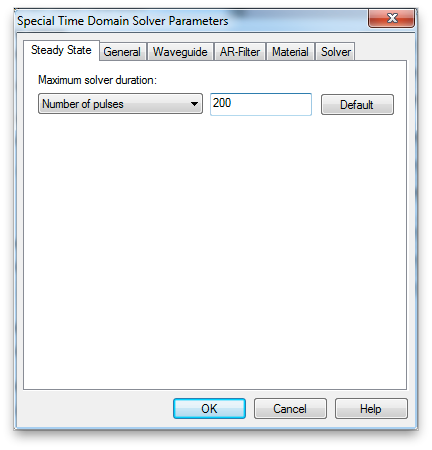
You may also find that the simulation terminates before reaching the desired accuracy. There is a default Maximum solver duration of 20 pulse widths (the transient time length of twenty times the excitation pulse width). I usually increase this to 200 if I am really willing to wait for the desired accuracy - which I usually am.

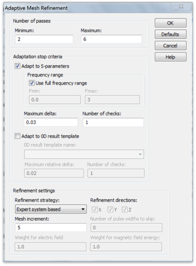
Simulate the WiFi/GPS/Bluetooth antenna first. From the Time Domain Solver Parameters panel, set the Source Type to Port 1 (the left side port). Set the Accuracy to -50dB and use Adaptive mesh refinement to find a good mesh, but open the Adaptive Mesh Refinement panel and set the Maximum delta to 0.03. We need to sacrifice some accuracy for speed to do the optimizations in this assignment.

Your refinement should stop after four passes. Turn off adaptive meshing when prompted.

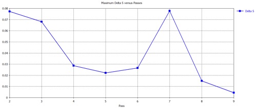
1. Compare your assumptions about mesh convergence that you would make after four passes and after nine passes. The maximum Delta S for nine passes is shown below. What advantages does the four-pass mesh have over the nine-pass mesh?

Now find the vertical position of the feed that will maximize the radiation. This is essentially impedance matching the antenna to the 50 Ohm waveguide represented by the discrete port. The load impedance of the antenna looks different depending on where we connect to it, i.e. the potential and current distribution of the resonant mode of the antenna leads to different ratios of potential to current at different locations.

Perform a parameter sweep of the vertical position of the discrete port from zero millimeters below the handset center to twelve millimeters below the handset center, in one millimeter steps.

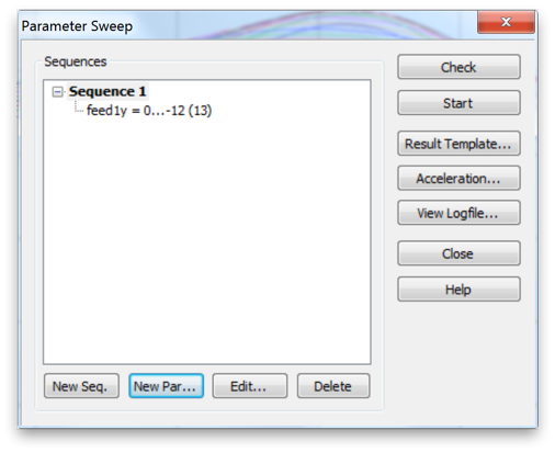
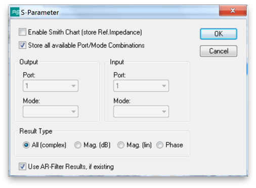
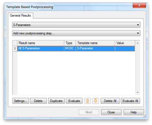
Click Result Template... to generate output for the sweep. Select S-Parameters from both menus, and check Store all available Port/Mode Combinations. Click OK.

Run the sweep and export the S-parameters from the Tables folder.

2. Now plot Pin/Pstim (the normalized input or accepted power) versus frequency for all thirteen sets of S-parameters.

Find the set that has the largest peak. Hopefully, this is a peak near our desired operating frequency of 2.4GHz (for WiFi and Bluetooth). That data set comes from the simulation with the (locally) optimal vertical position for the feed. (Assuming that the absorbed power is not dominating the results.) Also find (as precisely as possible) the frequency of the peak.

If your strongest peak came at an end point of your parameter sweep, perform another sweep that continues along the slot, until you find a local maximum.

3. 3.Report your optimal feed position and frequency.
   

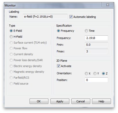
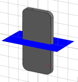
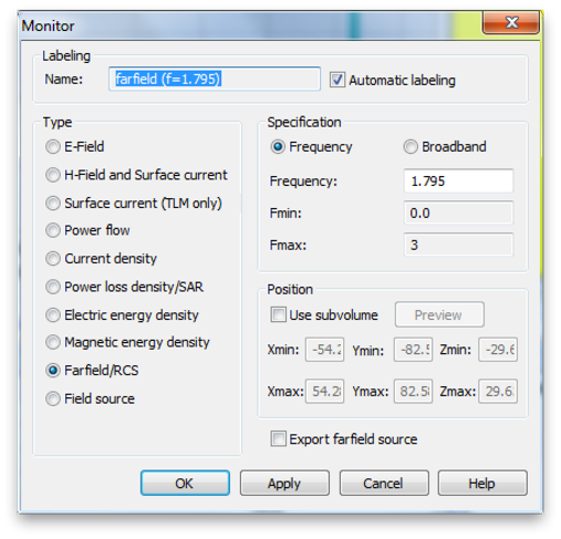
Now we will look at the near and far fields at this frequency and with the feed at this optimum position. Enter the optimum feed position into the appropriate variable of the Parameter list  table. Set three field monitors: E-field, H-field and Farfield/RCS. Select Field Monitor from the Simulation tab. In the Monitor panel, select E-Field. Enter the frequency of your Pin peak (2.1918 GHz for me), and Activate the 2D Plane. (The later saves a lot of file space.) Choose the Orientation and Position so that the field monitor will slice through middle of the handset as shown.

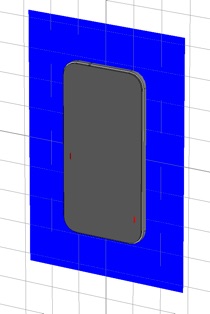
Create two H-Field monitors with 2D planes as shown. Also, create a Farfield/RCS monitor. (There is no 2D Plane option for the Farfield monitor.) All the monitors should be at the optimal frequency. Run the single simulation (not the paramter sweep.)

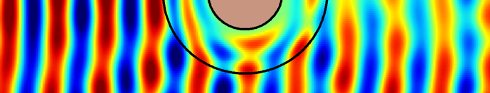
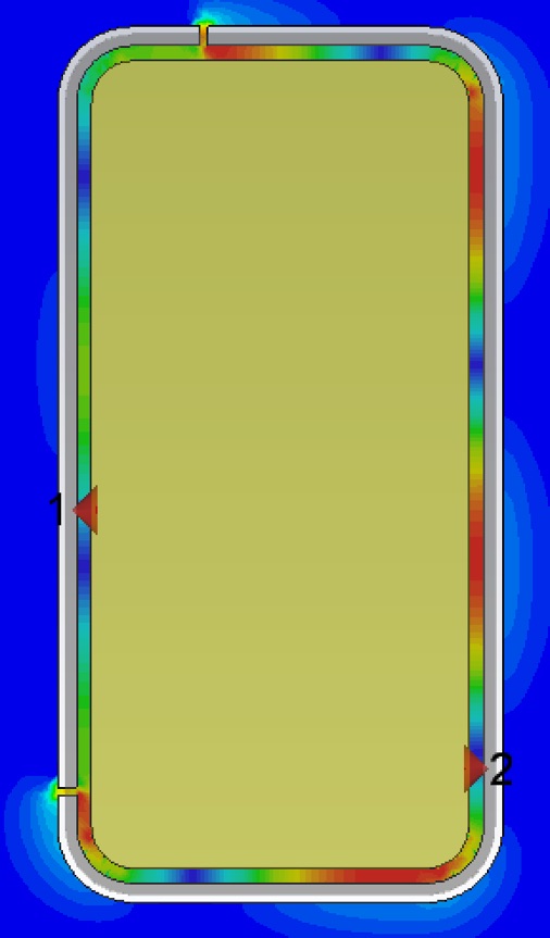
Examine the near fields. Select 2D/3D Results >> E-fieldr>>e-field (f=#.####;z=#)>>Abs in the Navigation Tree. Then get the contextual menu from the plot window (right click the mouse) and select Plot Properties... Check Plot Amplitude in the Phase/Animation area, and finally, click Specials... and check Clamp to range. Adjust the range to so that the full color map is used in the slot and not just at some small hot spots near the splits (due to auto scaling.)

E-field:

H field:

4. 4.Make similar plots from your own simulation. Qualitatively describe the number and locations of impedance maxima and minima along the slot (all the way around). At your optimized feed point, is the impedance relatively high or low?
   

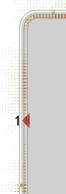
You can see the vector orientation of the fields by selecting the field result folder, instead of one of the contained components. You may need to play with the arrow density and scaling to get an informative view. You should animate the vector field plots to see the dynamics. Electric field is shown below on the left and magnetic field on the right.

5. 5.What type of wave is in the slot? Traveling clockwise, traveling counter-clockwise or standing? Can you tell how the magnetic field loops are oriented? Describe the direction of the current flow that generates these fields?
   

Now look at the linear efficiencies:

1 D Results>>Efficiencies>>linear

The radiation and total efficiencies are reported here. (You can get the numerical values of these two data points by selecting Show Axis Marker from the contextual menu of this plot.)

6. 6.At the Pin peak frequency, calculate all of the powers normalized to Pstim: Prefl, Ptrans, Prad, and Pabs. Are you satisfied with this antenna performance?
   

For the GSM (right side feed) antenna, give the built in optimizer a try. Before setting that up make some changes to our field monitors. Delete the E and H monitors and change the frequency of the Farfield monitor to 1.795 GHz. This is between the DCS-1800 uplink and downlink bands.  GSM Bands

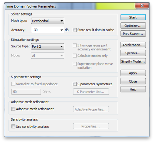
Also make some changes to the Time Domain Solver Parameters that will speed things up. (We will need to performs hundreds of simulations to do a good optimization.) Set the Accuracy to just -30. and the Source type to Port 2, since that is the port driving the antennas for the GSM radio.

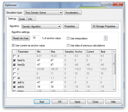
Now click the Optimizer... button. The two main ingredients in an optimization are the parameters and the goal function. First set the parameter space you want search. Pick the parameters that control the locations of both splits and both feeds, and give them a big range, but one that keeps them out of the corners. Also choose and algorithm. We want to do a global optimization, so choose one of the global algorithms: Genetic Algorithm or Particle Swarm.

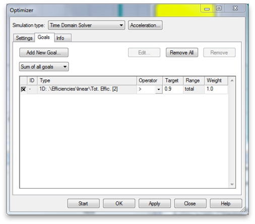
Now click the Goals tab to set up the goal function. We want to maximize the total efficiency with respect to Port 2. Shoot for greater than 0.9, or greater.

7. Get a screen capture of the Goal Value plot.

Note that the goal function is actually

goal = Target - Total Efficiency

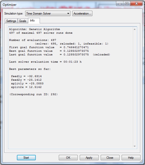
In this way , CST converts the maximization problem to a minimization problem with target of zero. I ran for about 10 hours and was able to get a Total Efficiency of 0.77.

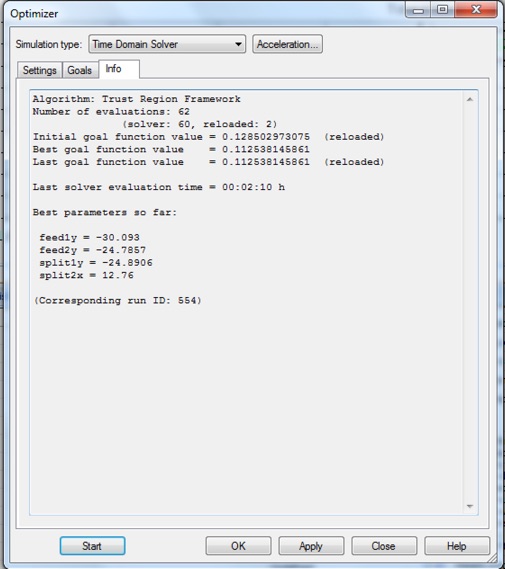
It is often a good idea to follow up a global optimization with a local optimization. Here I used the Trust Region Framework algorithm to get the Total Efficiency up to 0.79.

It’s worth taking a look at the radiation pattern too, which is available in the Farfields folder.

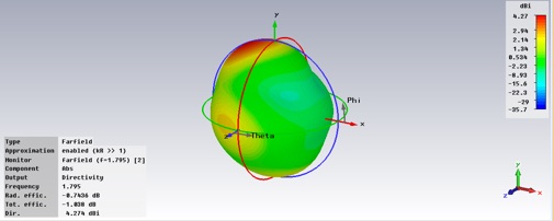
8. Calculate all the relevant powers as in 6, above, for the operating frequency 1.795GHz.

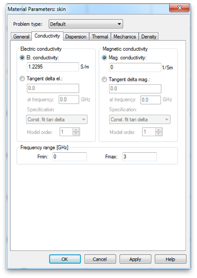
Now let us try to simulate the death grip. Get the electromagnetic properties of wet skin from this excellent website. In particular get the conductivity and the relative permittivity of wet skin at the operating frequency. (We will assume these properties are relatively constant over the GSM band.) Make a new material with these properties.

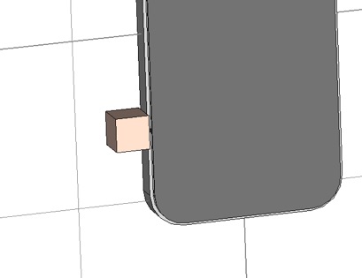
Put a cubic centimeter of this material centered on, and touching, the split. Re-simulate.

9. Calculate all the relevant powers as in 6 and 8. What is the drop in radiated power (in dB) induced by touching the split? Where is most of the power going, that is now not being radiated? Did the absorbed power go up or down? Why?