Assignment

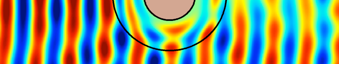
Simulate the ten different Split Ring Resonators (SRRs) in the article Metamaterial electromagnetic cloak at microwave frequencies.

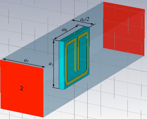
The units we have been using (mm, GHz and nS) are probably a good choice. A frequency range of 0 to 25GHz will include the important features of the magnetic and electric resonance. The boundary conditions should be chosen so that the magnetic flux of the TEM mode links the loop of the SRR.  If the SRR is oriented normal to the x-axis then the Xmin and Xmax boundaries should be magnetic. The Ymin and Ymax boundaries can then be chosen electric and the Zmin and Zmax boundaries open. Use open instead of open add space. Since we will need to add space around the resonator, we might as well add our own fixed amount of space for the ports.

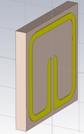
Set up the unit cell as shown below. All geometric parameters are given in the article. Use global variables for the geometric features, r and s, that vary for the different designs. It will also be convenient to use a global parameter for the metal thickness. Global parameters can be easily created by typing a valid variable name into the parameter entry fields when defining an object. You will then be prompted to enter a default value.

Start with the substrate so it will be easier to tell that the resonator ring is being located in the right place. Choose Rogers RT5870 (lossy) from the material library for the substrate and Copper (annealed) for the metal. Putting the origin at the center of the ring, and at the substrate-metal interface, may make constructing the ring easier, but other choices are fine obviously.

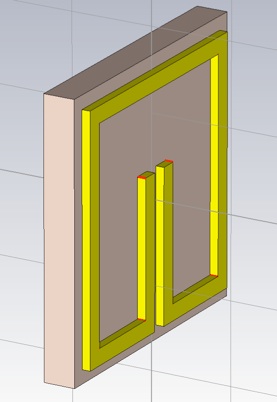
Construct the ring with square corners first then blend the edges later. You can draw a thin square slab for the ring and then cut out the center regions and gap (using appropriate bricks and boolean operations), or draw individual ring segments as bricks (making them into one object with Objects>>boolean>>Add). In the later case, you can use the Mirror operation under Objects>>Transform... to create half the object for you.

Now select the edges to be blended (keyboard shortcut is e). Select first the edges that will have the interior radius, r (some of which are not shown below). You may want to make the object thicker to make it easier to select the edges.

Perform the blend using Objects>>Blend edges... Then select the edges that will have the radius, r+w (to maintain a constant cross section in the corners).

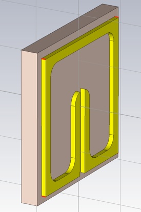
Perform the blend and return the object to its desired thickness of 0.017 mm.

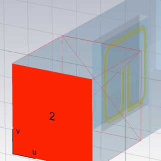
Now add some vacuum around the SRR, including perhaps a unit cells length of space between the substrate and where the ports will go. To resolve the intersecting shapes, you will need to trim highlighted shape for both the SRR and the substrate. You may want to make the Vacuum material transparent so you can see the SRR even when it is not selected. (Double click Material>>Vacuum in the Navigation tree to do this.)

Add the ports and be sure to adjust the port reference to the edge of the substrate.

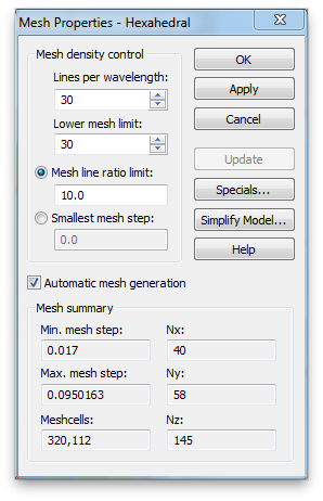
The Adaptive mesh refinement will not give a satisfactory result for reasons I will explain in class. You should use 30/30 (or higher) in the Mesh density control (Mesh>>Global Mesh Properties..).

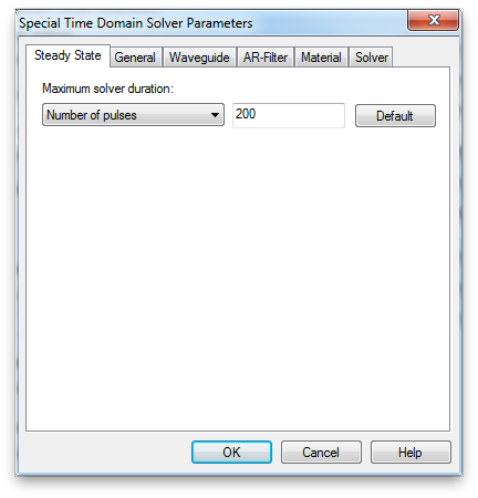
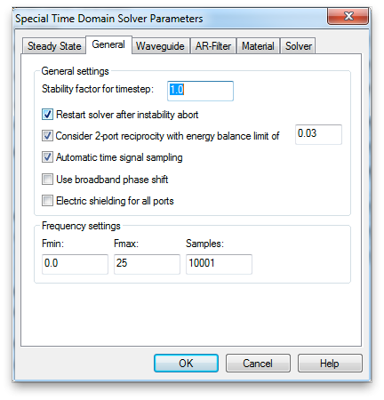
Open the transient solver panel. As usual, use -50dB for the accuracy and set the source type to port 1 only. Click the Specials... button to bring up the Special Time Domain Solver Parameters panel. Select the Steady State tab if it is not already selected. You need to extend the steady state time out condition. The simulation will not ready the -50dB accuracy in 20 pulses. Make it 200 to ensure the simulation will run to the -50dB energy level. Click OK.

Then select the General tab. For the sharp resonances we will see in the S-parameters, it would be better to have more samples in your frequency range. Increase the Samples to 10,001. The frequency interval will then be 25GHz/10000 = 2.5 MHz.

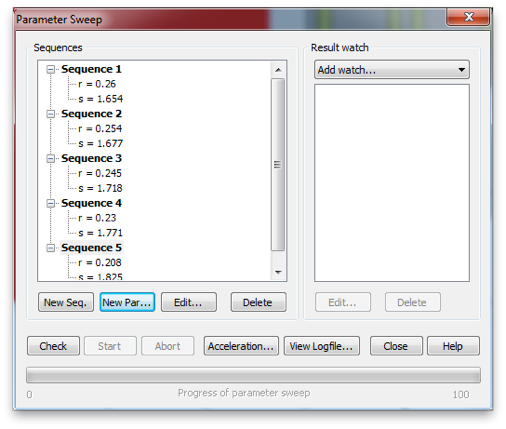
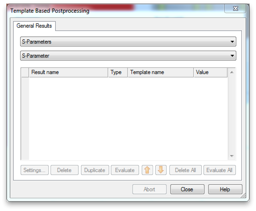
Then select Par. Sweep... to set up the simulation of all ten unit cell designs. Referencing your global parameters create a sequence for each design, adding the two parameters, r and s, with appropriate values for each. Then use Add Watch>>Processing Template... to create the result watches for S-Parameters.

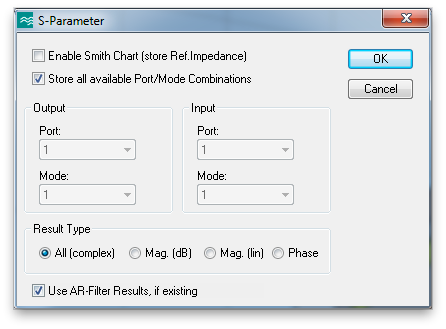
Select S-Parameter from the second menu.

Click Start in the Parameter Sweep window to begin the simulations. It might take two or three hours to run all ten.

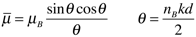
Export the S-parameters. If you can export each of the two data tables to separate files, while using the Polar display, you will have all of the S-parameter data. Extract the material properties epsilon and mu. Note that a-theta is the correct extraction thickness. You will probably not need to adjust the branch choice to obtain the correct results. Generate a plot for epsilon and a plot for mu. In each, plot the real part of the ten extracted material properties versus frequency. Zoom the plot to display the region around the operating frequency, which we will take to be 8.55 GHz. Also plot the real part of epsilon and mu versus radius, r, in the cloak at the operating frequency. The formula relating cloak radius to cylinder number is

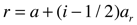
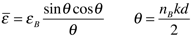
where a is the cloak inner radius (given in the article), i is the cylinder number and a-r is the radial unit cell dimension (also given in the article). In this plot versus radius, also include the desired analytical expressions for the material properties. These are given in equation (3) in the article. Submit the four plots.

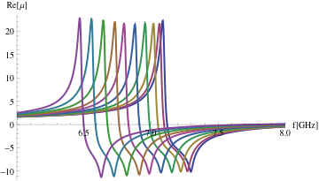
You may have noticed that the permittivity resonances (around 20 GHz) and the permeability resonances (around 7 GHz) have distinctly non-Lorentzian shapes.

There are ways to get at the underlying Lorentzian material resonance from the S-parameter extracted properties (which are modified by spatial dispersion due to the finite unit cell size and the non-uniform distribution of polarization across the unit cell).

Smith has a more recent article on metamaterial properties that gives formulas for doing just that. See equation (24) and (31).

For the permittivity resonances use the following equation to calculate the underlying Lorentzian material properties.

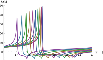
where the B-subscripted properties are the ones you have obtained via extraction from the simulated S-parameters. (B stands for Bloch.) The quantities with the bar are the underlying (or averaged) properties. On one graph, plot the real part of the averaged permittivity for all ten designs in the frequency range 16 - 23 GHz.

For the design of cylinder one, fit the averaged complex permittivity to the Lorentzian function.

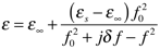
Report the four fitting parameters, and plot the real and imaginary parts of the permittivity for both the simple Lorentzian function (with your best fit parameters), and the extracted averaged permittivity.

Here is an example of least squares curve fitting with Matlab. Also, here are some MATLAB files I wrote to fit some data to a lorentzian: test.m fitfun.m lorentzian.m. Note, the Lorentzian function in this code is for the engineer’s time harmonic convention (where there is a negative imaginary part for material properties). If you are using the physicists time harmonic convention, and your permittivity and permeability data with a positive imaginary part. The fit will not work. You will need to be consistent with your time harmonic convention.

The Lorentzian and other material response models are described in the CST documentation:

CST MICROWAVE STUDIO>>Creating and Visualizing Models>>Material Overview (HF)

Do the fitting and plotting as above for the permeability resonances in the frequency range 6-8 GHz, using the equivalent formula for a permeability resonance

Lorentzian resonance functions are the characteristic response of second-order, damped harmonic oscillators, so they come up all the time, from LCR circuits to mechanical suspensions. Really, it’s the only problem you solve completely. To learn more about the Lorentzian response, explore with my Dipole Demonstration.