Assignment

In this assignment, we will find the S-parameters of a slab of brain grey matter by performing a time domain simulation. We will find these S-parameters with the default phase reference (incorrect) and with the phase reference de-embedded to the brain-vacuum interface (correct). Then we will compare the simulation results with an analytical formula.

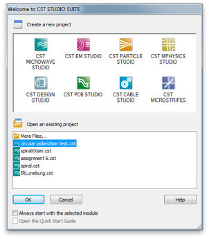
Launch CST Studio Suite (from the desktop.) Accept the university version agreement.

Then select CST Microwave Studio, the icon in the upper left corner.

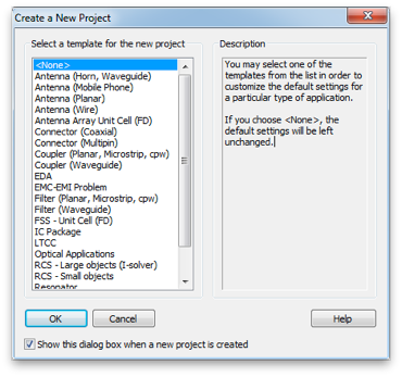
Then select <None> for the project template and click OK.

Generally, one works down the Solve menu, performing most of the tasks in menu order, culminating in running one of the solvers.

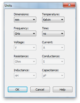
Select Units... from the Solve menu. Set the units to mm, GHz and ns (nano-seconds). These will be most convenient units for the scale we will be working at.

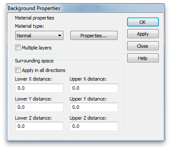
Select Background Material... from the Solve menu. Set the background material to Normal and leave Epsilon and Mue at unity. These are the material properties relative to vacuum. So we are setting the background material to vacuum. (Note that the properties of air are very close to vacuum.)

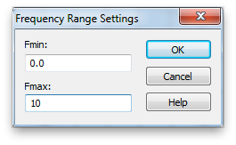
Skip Materials for now, and set the maximum frequency to 10 GHz.

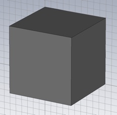
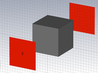
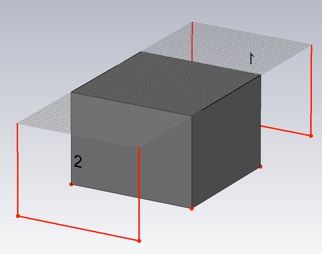
Use the Create brick tool to create a cube of brain grey matter, 10mm on side. The tool is a small cube in the tool bar.

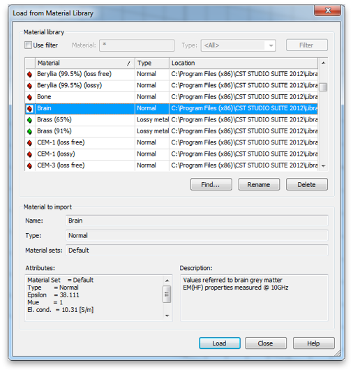
Hit escape to pull up the numerical entry panel. Set the dimensions as shown and select [Load from Material Library...] from the Material: menu. Load the lossy Teflon from the material library as shown.

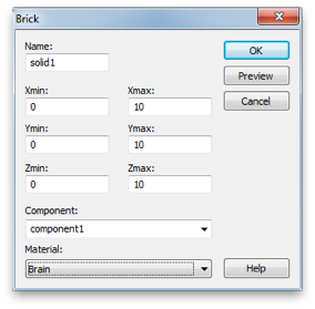
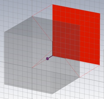
The brain cube.

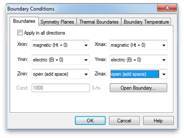
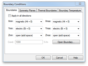
Set the boundary conditions to magnetic (Ht=0) on the two X-planes, electric (Et=0) on the two Y-planes and open (add space) on the two Z-planes. This creates a TEM waveguide, something difficult to do in the lab, but easy in simulation.

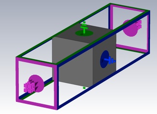
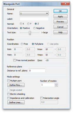
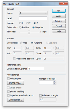
Skip down to Waveguide Ports... and create two waveguide ports. Use all default values, except choose Negative orientation for the second one.

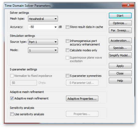
Select the Transient solver... and set the accuracy to -50 dB, the source to Port 1 and check the Adaptive mesh refinement box. Start the simulation.

Watch the convergence by viewing: 1D Results>>Adaptive Meshing>>|S| linear>>S21 or S11 from the Navigation Tree, on the left. The default view is the real part of the S-Parameter.

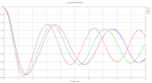
The simulation stops when the S-parameters converge. You will be asked if you want to disable further adaptive meshing. Select ‘yes’.

To export the magnitude and phase of both S-parameters first display them in polar form. Right click S-Parameters from the Navigation Tree, and select Plot View and then Polar. (You can also change the view with view icons in tool bar.)

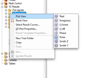
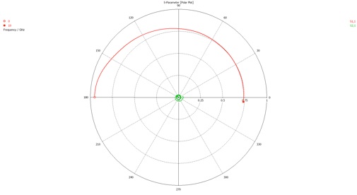
Now export the ascii data using FIle>>Export>>Plot Data (ASCII).... The file should look like this:

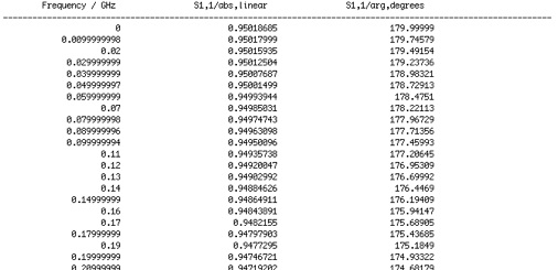
Load the data into your favorite analysis package (e.g. MATLAB or Mathematica). Plot the linear magnitude of S11 and S21 (second column of file) versus frequency (first column of file). (Note that the S11 data is at the top of the file and the S21 data begins half way down.) Make sure this plot looks like the plot you get when you select | | linear from the Plot View menu.

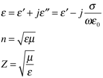
For the gray matter material, the imaginary part of the permittivity is represented as a conductivity. The complex (relative) permittivity and its relationship to the refractive index and impedance are given by

1. 1.Now plot the corresponding analytical result using equation 1 and 2 of this article, in the same graph. Adjust the styles and/or point density so both the simulation and analytical results can be clearly seen. Note that in the article r corresponds to S11 and t prime corresponds to S21.
   

Now lets see if the simulation and analytical results agree in phase as well as magnitude.

2. 2.On one graph plot the real and imaginary parts of S11 versus frequency, both from simulation and equation 1 and 2. (Make sure you convert either the data or the equations so that both use the same time harmonic function convention.) Make a second graph of this type for S21.
   

3. 3.Explain why these results do not show agreement between simulation and analytical results.
   

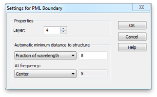
Now we will fix the problem by de-embedding the simulation S-parameters. We will accomplish this by shifting the port reference planes. The open (add space) boundary assignment has added some background media of thickness equal to one eighth of the wavelength (in the background medium) at the center frequency (5 GHz). You can check or change these settings by clicking the Open Boundary... button in the Boundary Conditions panel.

Now open the Waveguide Port panel by double clicking a port in the Navigation Tree.

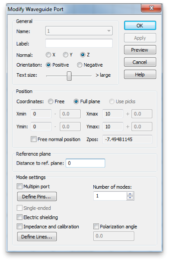
Enter the correct value in the Distance to ref. plane box. (You may enter an expression that uses arithmetic operators if you like.) A negative value moves the reference plane in toward the Teflon block. Make sure the reference plane lies on the block as shown.

Do the same for the other port, then re-run the simulation and export the data.

4. 4.Re-do the graphs, as in 2 above, with the new data.
   

5. 5.How is the agreement now?
   

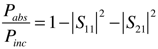
6. 6.Finally calculate the fraction of the incident power that is absorbed in the gray matter and plot it versus frequency.
   

7. Do you expect that your cortex or hippocampus absorbs more microwave energy from you phone? Why?