Invisibility Cloak

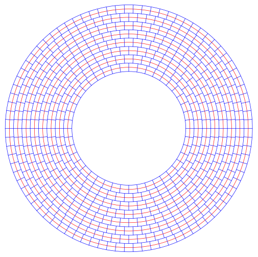
Simulate the ten different Split Ring Resonators (SRRs) in the article Metamaterial electromagnetic cloak at microwave frequencies.

Start a new CST Microwave Studio project by clicking Project Template. Then select MW&RF&Optical, Periodic Structures, FSS, Metamaterial - Unit Cell., and Phase Reflection Diagram. Then choose Time Domain; we will be doing normal incidence.  The default units will be good for the scale we will work at. A frequency range of 0 to 25GHz will include the important features of the magnetic and electric resonance. Don’t check the Calculate reflectance, transmittance, absorbance box. Then Finish on the next panel.

We will change the boundary conditions that this template set up. Open the Boundary Conditions panel. The boundary conditions should be chosen so that the magnetic flux of the TEM mode links the loop of the SRR.  If the SRR is oriented normal to the x-axis then the Xmin and Xmax boundaries should be magnetic. The Ymin and Ymax boundaries can then be chosen electric and the Zmin and Zmax boundaries open (add space). (Don’t worry about the calculation domain warning. CST just does not know yet, how large of objects we plan to create.)

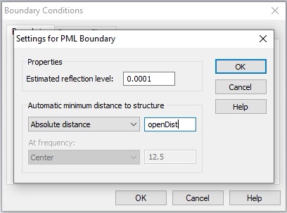
Select the Open Boundary... button and choose Absolute distance from the Automatic minimum distance to structure menu. You should get in the habit of using global parameters. Global parameters can be easily created by typing a valid variable name into the parameter entry fields when defining an object. You will then be prompted to enter a default value. Choose an appropriate parameter name and set the value to 3mm. You can use this variable later when you set the distance to reference plane for the ports.

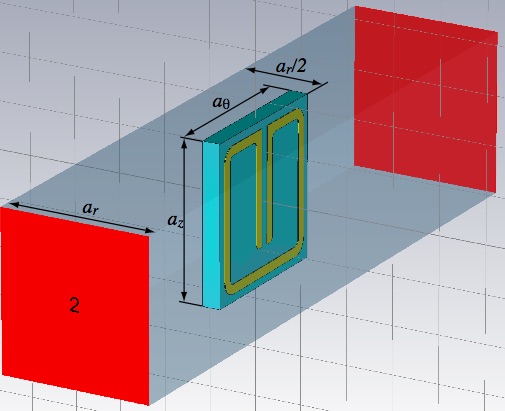
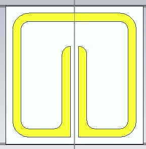
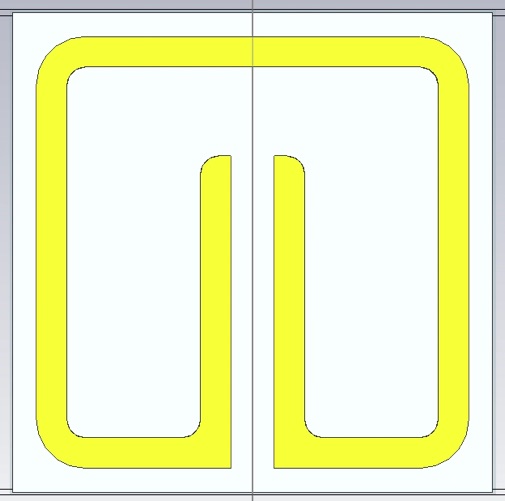
Set up the unit cell as shown below. All geometric parameters are defined in the article linked above. Use global parameters for the geometric features, r, s, w, and, g (the horizontal gap between the two vertical traces in the center of the unit cell). For the initial values use:

r = 0.2 mm

s = 2 mm

w = 0.2 mm

g = 0.2 mm

It will also be convenient to use a global parameter for the metal thickness. (The r, θ, z subscripts here refer to the cylindrical coordinates of the cloak and not the cartesian coordinates of CST. You should put the ports normal to the CST z-axis.

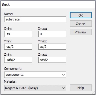
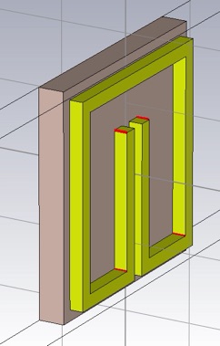
Start with the substrate so it will be easier to tell that the resonator ring is being located in the right place. Choose Rogers RT5870 (lossy) from the material library for the substrate and Copper (annealed) for the metal. Putting the origin at the center of the ring, and at the substrate-metal interface, may make constructing the ring easier, but other choices are fine obviously. For that choice, the substrate brick might look like this

Construct the ring with square corners first then blend the edges later. You can draw a thin square slab for the ring and then cut out the center regions and gap (using appropriate bricks and boolean operations), or draw individual ring segments as bricks (making them into one object with Modeling>>Boolean>>Add). In the later case, you can use the Mirror operation under Modeling>>Transform to create half the object for you.

Now select the edges to be blended (keyboard shortcut is e then double-click the edge). Select first the edges that will have the interior radius, r (some of which are not shown below). You may want to make the object thicker to make it easier to select the edges.

Perform the blend using Modeling>>Blend>>Blend edges... Then select the edges that will have the radius, r+w (to maintain a constant cross section in the corners).

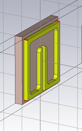
Perform the blend and return the object to its desired thickness of 0.017 mm.

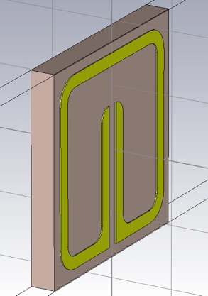
Check the Right view (6).

Now add some vacuum around the SRR. This should be a block that is ar by az by aθ.

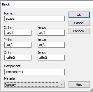
To resolve the intersecting shapes, you will need to trim highlighted shape for both the SRR and the substrate. You may want to make the Vacuum material transparent so you can see the SRR even when it is not selected. (Double click Materials>>Vacuum in the Navigation Tree to do this.)

Add the ports and be sure to adjust the port reference to the edge of the substrate.

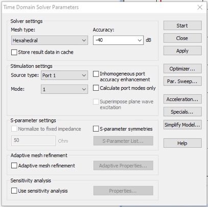
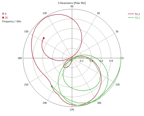
Do a quick simulation with the default Mesh and Accuracy. Choose to excite just Port 1, since by reciprocity S12 = S21, and by symmetry S22 = S11.

When the simulation is complete, display both S-parameters in the polar format. Your results should look pretty much exactly like the plot below and take about 30s.

I found that this optimization did not work for me unless the CST files were on the local hard drive of the simulating processor. I strongly suggest you move your model file to the local drive. You can copy it back to your Engman home directory as needed.

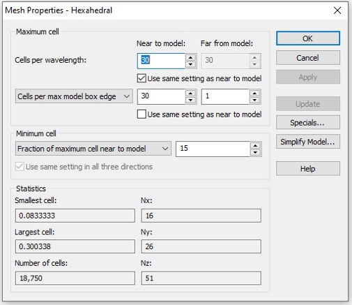
Now let’s make some changes for improved accuracy. The Adaptive mesh refinement will not give a satisfactory result for reasons I will explain in class. You should use 30/30 in the Mesh density control (Simulation>>Mesh>>Global Properties).

Set the Accuracy to -60dB.

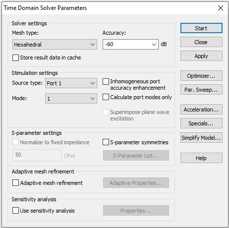
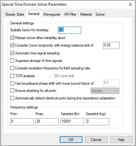
Then select Specials... and then the General tab. For the sharp resonances we will see in the S-parameters, it would be better to have more samples in your frequency range. Increase the Samples to 10,001. The frequency interval will then be 25GHz/10000 = 2.5 MHz.

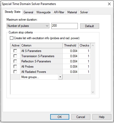
Click OK. Next select the Steady State tab. You need to extend the steady state time out condition. The simulation will not reach the -60dB accuracy in 20 pulses. Make it 200 to ensure the simulation will run to the -60dB energy level.

Click OK, and close the Time Domain Solver Parameters panel.

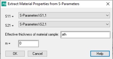
For this assignment we will use the built in material property extraction template (but don’t forget that you know how to do it yourself). Open the Template Based Postprocessing panel from the Post Processing tab. Choose S-Parameters and then Extract Permittivity and Permeability from S-Parameters from the menus. Enter your variable for a-theta in the Effective Thickness of material sample field, and click OK. Close the Template Based Postprocessing panel.

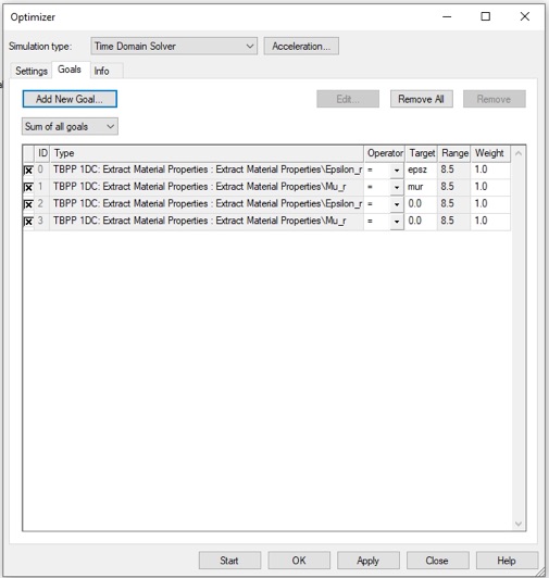
Open the Optimizer, and set up the parameter settings for the: gap (g), radius (r), capacitor length (s) and trace width (w) as follows. Don’t use just the 10% default rage for the parameters.

We can use a local optimizer, like the Trust Region Framework. Next set up the goals to target the real parts of epsz and mur that you have been assigned. We also want the imaginary parts to be as small as possible.

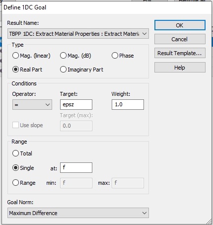
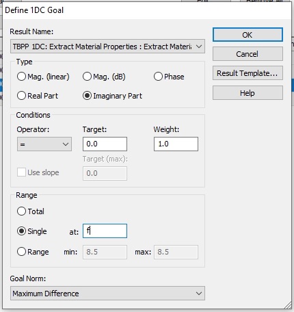
We want the operating frequency to be 8.5 GHz. Make goals for mur too.

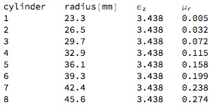
The target values depend on the cylinder number that you were assigned.

Now you can run the optimizer and let it run to completion.

Our goal is to get the real parts pretty much dead on, and the imaginary parts as small as possible. Try for the following:

If you can’t reach these goals just running a local optimization from the initial parameter values. Try running a global optimization for a while and then use the best parameter values for a follow on local optimization.

Copy the best values of the four fit parameters to some place safe. Also get the best values for the real and imaginary parts of epsz and mur at the operating frequency (8.5 GHz), and a screen grab of the metamaterial unit cell viewed straight on (i.e. Right view).

Also, send me a message with your cylinder number, and your best values for the real and imaginary parts of epsz and mur at the operating frequency (8.5 GHz).

In the report:

1. 1.Provide the best fit values of the four geometric parameters: g, s, w, r. Include a screen grab of the unit cell, like the one above, dimensioned with these parameters (i.e. with arrows and reference lines showing the definitions of the parameters.)
   

2. 2.For g, s and r, state what effect each has on the real part of εz or μr. Is there a positive or negative correlation? For each positive or negative correlation explain using the intermediate quantities: capacitance, resonance-frequency, proximity-to-a-negative-or-positive-resonant-response.
   

3. 3.Provide the optimized complex valued material properties, εz or μr.