Metamaterials: Effective Media

In this assignment, we will find the S-parameters of a slab of polycarbonate plastic by performing a time domain simulation. We will find these S-parameters with the default phase reference (“incorrect”) and with the phase reference de-embedded to the polycarbonate-vacuum interface (“correct”). Then we will compare the simulation results with an analytical formula.

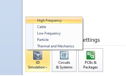
Launch CST Studio Suite (from the desktop.) Accept the university version agreement. At the bottom of the screen, select High Frequency from the 3D Simulation menu.

This puts you into the most general Maxwell’s equations solver environment. You can also use templates to preselect some of the settings for a specific problem type. Here we will start from the generic defaults.

We must set up a few basic things, before we do any modeling.

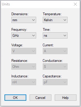
Click the Home tab, then click Units on the command ribbon. Set the units to mm, GHz and ns (nano-seconds) and click OK. These will be the most convenient units for the scale we will be working at.

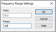
Next select the Simulation tab, and click Frequency.  Set the minimum frequency to 0.1 GHz, and set the maximum frequency to 60 GHz.

Click Background. Set the background material to Normal, instead of PEC. The values for the background Epsilon and Mue can be adjusted using the Properties... button, but just leave these values at unity. In CST, Epsilon and Mue refer to the material properties relative to vacuum. So we are setting the background material to vacuum. (Note that the properties of air are very close to vacuum.)

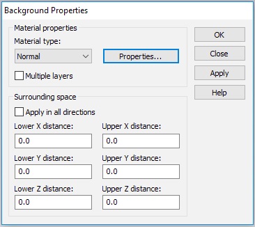
It’s a common mistake to omit this step and not realize that all the undefined regions in your simulation would then be the default, PEC, a perfect electric conductor.

Now select the Modeling tab. Use the Brick tool to create a cube of polycarbonate, 3mm on a side. The tool is a small cube on the command ribbon.

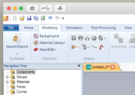
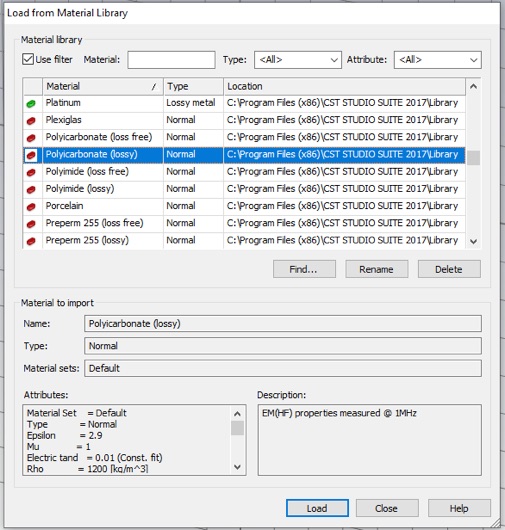
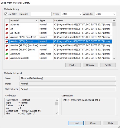
Hit escape to pull up the numerical entry panel. Set the dimensions as shown to create a 3mm cube and select [Load from Material Library...] from the Material drop down menu. Load Polycarbonate (lossy) from the material library as shown.

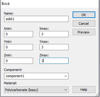
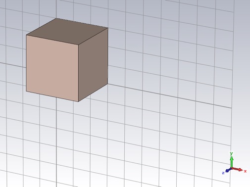
Click OK to see the polycarbonate cube.

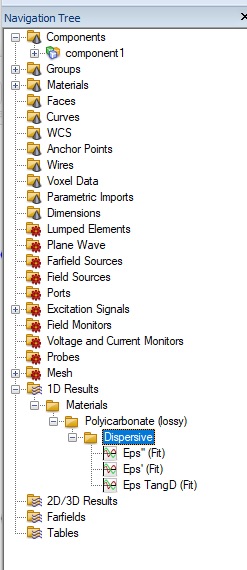
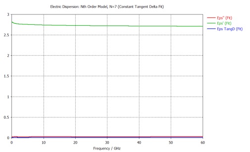
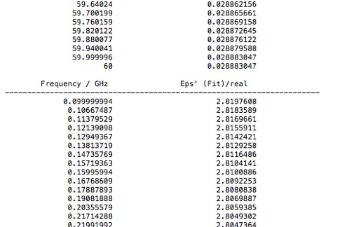
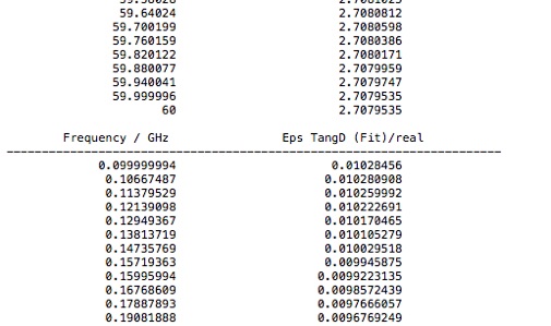
You can display the frequency-dependent polycarbonate material properties by selecting the them from the Navigation Tree.

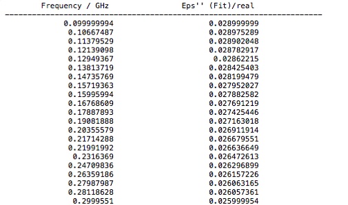
You will need this property data for analysis. One way to export it, is to select the Post Processing tab and select Export>Plot Data (ASCII)... from the Import/Export menu. All three data sets will be stored in the same file. Check that it looks like the file below. Three locations in the file are shown. There are three headers in this file. One at the start of each material property data set.

Alternatively, one could cut and paste that data into, for example, an Excel spreadsheet, or directly into MATLAB, using the Paste Special  from the Edit menu.

Note, that CST uses the engineers’ convention for the time dependence of harmonic functions

and not the physicists’ convention

so that, for example, passive materials have a negative imaginary part. However, CST uses the primed and double primed symbols to represent the real and negative imaginary part of a complex quantity

Also, tanδ is usually considered to be a positive quantity for passive materials, regardless of convention.

tanδ is a commonly specified material property that gives a measure of the lossiness of a material.

You can return to the 3D cad layout by clicking the 3D tab below the display window.

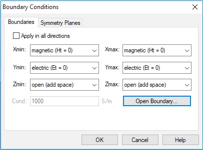
Next go back to the Simulation tab, and click Boundaries. Set the boundary conditions to magnetic (Ht=0) on the two X-planes (i.e. Xmin and Xmax), electric (Et=0) on the two Y-planes and open (add space) on the two Z-planes. This creates a TEM waveguide, something difficult to do in the lab, but easy in simulation.

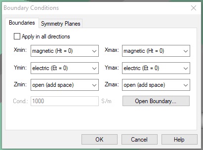
If you re-open the Boundaries panel, all the set boundaries will show color coded as follows.

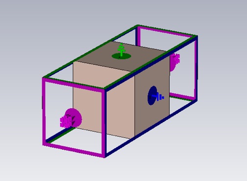
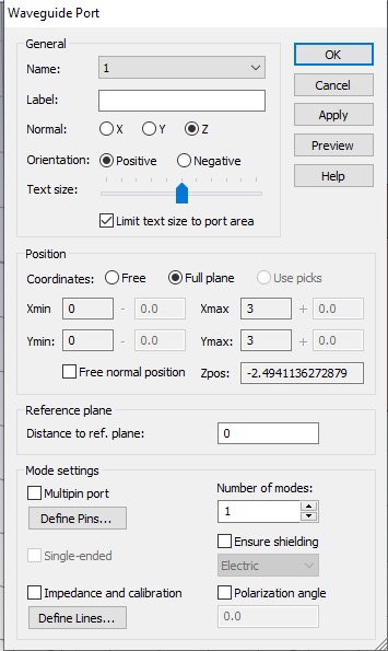
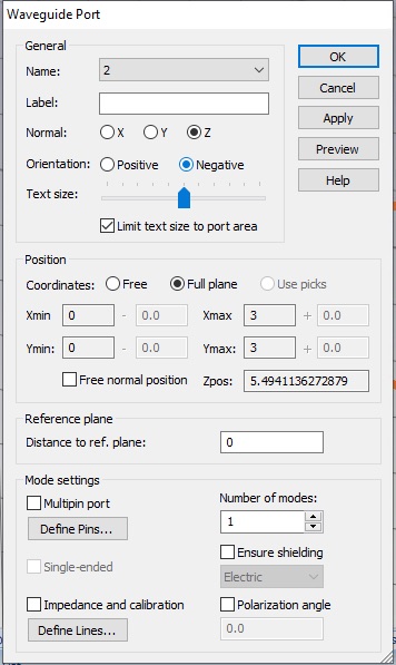
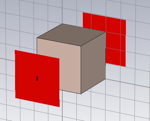
By clicking Waveguide Port, create two waveguide ports. Use all default values, except choose Z Normal  for both ports and and Negative orientation for the second one.

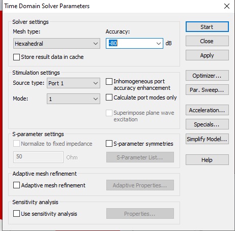
Now click Setup Solver, which will open the Time Domain Solver by default. (You can select other solvers on the Home tab.) Set the Accuracy to -50 dB, the Source Type to Port 1 and check the Adaptive mesh refinement box.

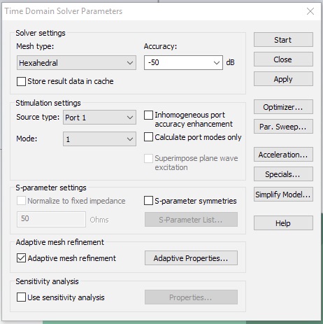
Adaptive mesh incrementally increases the mesh to check for convergence. Let’s set a very strict convergence criteria, so we can observe the process over several passes. Click the Adaptive Properties... button. Set the Maximum delta to 0.004.

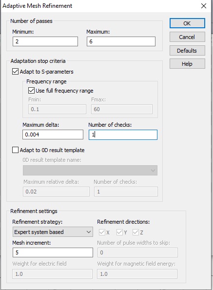
Click OK, then click Start in the Time Domain Solver Parameters panel to begin the simulation.

Click Mesh View, so you can watch the adaptive mesh refinement as it proceeds.  Ty different mesh view options to visualize the 3D structure of the mesh. Note that at the beginning of each simulation, the ports are adaptively meshed before the volume is simulated.

You can also watch the Port signals or Energy plots to see the approach to the simulation stopping criterial. These are both found in the 1D Results folder of the Navigation Tree.

After the mesh adaptation is complete, you will be asked to deactivate adaptation.

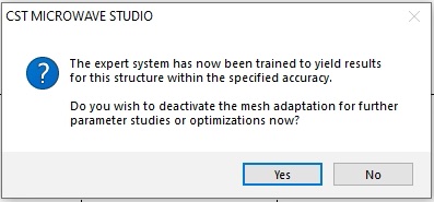
Click Yes. This will uncheck the Adaptive mesh refinement box, so that further mesh refinement will not occur in subsequent simulations.

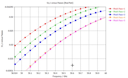
Look at the various results in the Adaptive Meshing folder, to see the consequences of the mesh refinement. If you zoom in to one of the S-parameters you will note that the Mesh Pass 4 and 5 are closer together than previous pairs of results. The S-parameters are converging to each other, and most likely to the result of an infinitesimally fine mesh -  this is the same as solution to the continuous differential equations which the finite-difference equations are approximating.

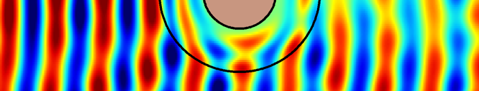
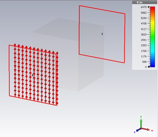
The S-parameters represent the amplitude and phase of the reflected and transmitted waves relative to the incident wave. The waves in question are the modes of the ports. It is very important to always look at the port modes to see if they are as you think.

From the Navigation Tree select 2D/3D Results>>Port Modes>>Port 1>>e1. (Also look at h1 as well as Port 2.)

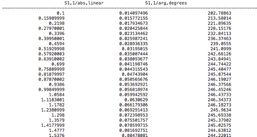
By displaying the S-parameters in polar form you will be able to save the complex values to a file. Select the S-Parameters folder from the Navigation Tree (not the ones inside the Mesh Adaption folder). These are the results from the last (and best) adaptation pass. Now click Polar from the command ribbon.

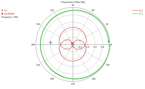
Then click the Post Processing tab and save the data as before. The file should look like this.

Load the data into your favorite analysis package (e.g. MATLAB, Mathematica or Python/numpy/scipy).

1. 1.Now plot these simulation results together with the corresponding analytical result for the S-parameters using equation 1 and 2 of this article and the material properties for polycarbonate that you exported from CST. For each S-parameter, put the curves for the simulation and analytical results in the same graph for comparison. To display these complex parameters, plot the real and imaginary parts as separate curves. Adjust the styles and/or point density so both results can be clearly seen.
   

Note that the article above is a physics article so that coefficients r and t’ are related to S11 and S21 through the complex conjugate

The wave vector, k, in equation 1 and 2 is the free space value and the speed of light in the units we are using is about 300.

Also, d, is the thickness of the material, which is in our case 3mm. The refractive index, n, and the relative impedance, z, are related to the relative permittivity, ε, and the relative permeability, μ, in the usual way

2. Explain why these results do not show agreement between simulation and analytical results.

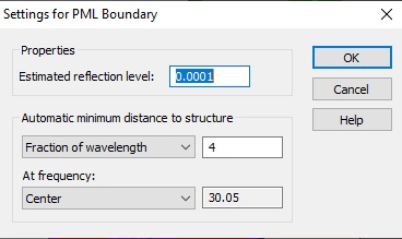
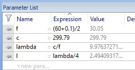
Now we will fix the problem by de-embedding the simulation S-parameters in a way consistent with our theoretical calculation. We will accomplish this by shifting the port reference planes. The open (add space) boundary assignment has added some background media of thickness equal to one fourth of the wavelength (in the background medium) at the center frequency (30.05 GHz). You can check or change these settings by clicking the Open Boundary... button in the Boundary Conditions panel.

Now open the Waveguide Port panel by double clicking a port in the Navigation Tree.

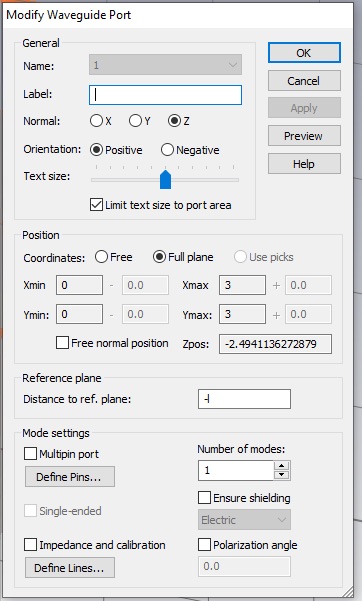
Enter the correct value or a global parameter in the Distance to ref. plane: box. I used global parameters to create the distance variable, l. Note that the to move the reference plane inward, the value should be negative.

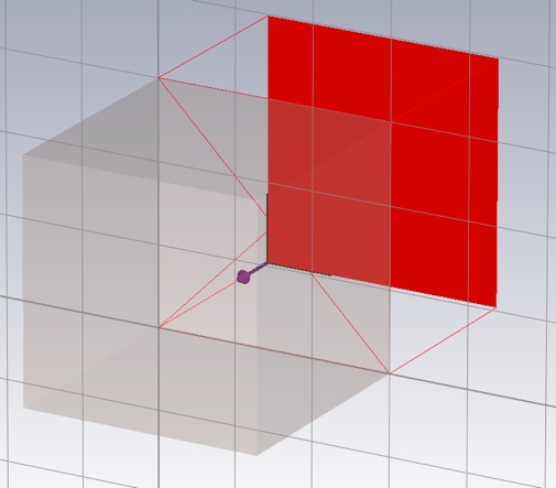
You may also enter an expression directly into the Distance to ref. plane box if you like. A negative value moves the reference plane in. Make sure the reference plane lies on the block as shown.

Do the same for the other port, then re-run the simulation and export the data. (The current mesh is fine. You don’t need to re-run the adaptive meshing, so keep that box unchecked.)

3. 3.Re-do the graphs, as in 1 above, with the new data. How is the agreement now?
   

Now that we have good agreement between our analytical model and simulation, we might be able to use the inverse analytical model to “extract” the material properties from the S-parameters. The Smith article provides the necessary equations.

4. 4.Using the S-parameters (S11 and S21) from the correctly de-embeded simulation, first calculate n and Z, and then μ and ε.  Submit plots comparing the real and imaginary part of the extracted μ and ε with the corresponding model material properties used in the simulation (which you have already exported). Make one set of plots using the built in inverse cosine function, acos, (i.e. without branch corrections), and one set of plots with the provided holomorphic inverse cosine function (i.e with branch corrections). (For μ the model properties are 1+0*j, since polycarbonate is non-magnetic )
   

Note this code works best when

function [ w, s, p ] = acosH( z )

s = ones(size(z));

p = zeros(size(z));

w = complex(zeros(size(z)),0);

w(1) = acos( z(1) );

for i = 2:size(z),

    a = acos( z(i) );

    pp = round( (w(i-1)-a)/(2*pi) );

    pm = round( (w(i-1)+a)/(2*pi) );

    wp = a + 2*pi*pp;

    wm =-a + 2*pi*pm;

    if abs( wp-w(i-1) ) <= abs( wm-w(i-1) )

        w(i) = wp;

        p(i) = pp;

        s(i) = 1;

    else

        w(i) = wm;

        p(i) = pm;

        s(i) = -1;

    end

end  

end

5. 5.How is the agreement between the material properties from the model, and those calculated using the inverse relations on the S-parameters obtained from simulation? Is the agreement better or worse than the agreement found for the S-Parameters. Try to improve the agreement by increasing the Accuracy parameter in your simulation, from -50dB to perhaps -80dB. (You can include just plots using the  more accurate simulation results.) At what frequencies is the agreement worst? What characteristic of the S-Parameters at those frequencies might explain this?
   

Now we will use the inverted theory, and extract material properties from S-parameters for a metamaterial with unknown properties, polycarbonate with spherical alumina inclusions imbedded in it.

We will simulate just one unit cell of the proposed material, and the boundary conditions will ensure (in this case) that we are finding the behavior of an infinite mono-layer of this composite.

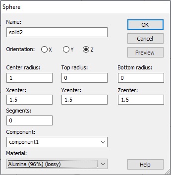
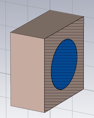
To insert an alumina sphere into the polycarbonate, click the Sphere tool, from the Modeling Tab. Hit escape to bring up the Sphere panel. Define a sphere of 1mm radius located in the center of the polycarbonate block. Choose the material, Alumina (96%) (lossy), from the Material menu.

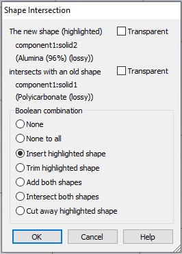
We now have material properties doubly specified where the spleen and water overlap. CST wants to know how to resolve this. Choose Insert highlighted shape.

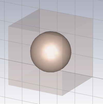
If you select the sphere object or its material in the Navigation Tree, you should see the following.

It might be helpful for visualization to make the alumina material a different color. If you double click a material in the Materials folder of the Navigation Tree, you can change it’s properties.

To verify the sphere is centered in the block you can rotate the block or use a Cutting Plane on the View tab.

Even though we have made substantial changes, the current mesh and solver settings should be fine, Run the simulation again and export the S-parameters. Also, export the material properties of the alumina, as we did before with the polycarbonate.

7. 7.Plot the real and imaginary parts of the permittivity and permeability as calculated from the S-parameters (using branch correction i.e. using the holomorphic arc-cosine) and from the Maxwell-Garnett theory, which can be found in the Resources section of the class website or in Wikipedia. As above, plot in such a way that the simulation derived results and the analytical theory can be easily compared.
   

8. 8.Over what frequency range would describe the agreement as quantitatively acceptable.
   

9. 9.Calculate the effective medium parameter, λ/d, versus frequency. Use the wavelength in the medium which is reduced by a factor of the real part of refractive index. n , compared to the vacuum wavelength. What values of this parameter corresponded to quantitatively acceptable agreement.