Invisibility Cloak

Now lets try a COMSOL simulation of the cloak. (We can’t use CST because CST does not allow off diagonal elements of the permittivity and permeability tensors.)

From the Start Menu select COMSOL Multiphysics 5.3, and then (Classkit License) COMSOL Multiphysics 5.3, to launch the application.

Then select Model Wizard, and then 2D. We will use a 2D solver since the experiment was performed in a 2D waveguide environment.

Select Electromagnetic Waves, Frequency Domain (emw) from the Radio Frequency list, then click Add.

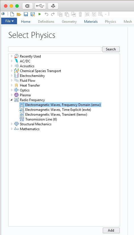
The cloak really only works well at one frequency, so a frequency domain solver will efficient.

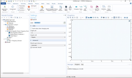
Now select Study, and choose the Frequency Domain study, then click Done. You should now see the three column workspace with: Model Builder, Settings, and Graphics.

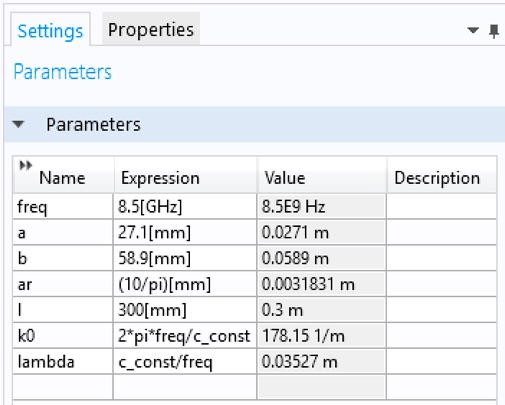
Now let’s create global parameters that we need. Right click Global Definitions and pick Parameters. Create the following global parameters.

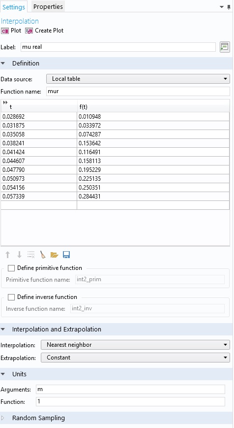
Now let’s create some functions from the CST data. Click Global Definitions in the Model Builder. From the Home tab, select Functions and then interpolation. Change  Data source: to File, and Browse... to your file called discretize. Then click Import. Change the Arguments: and Function: units to meters, m. Change the Label to discretize and the Function name to dis. Change the Interpolation: and Extrapolation: to Nearest Neighbor and Constant, respectively.

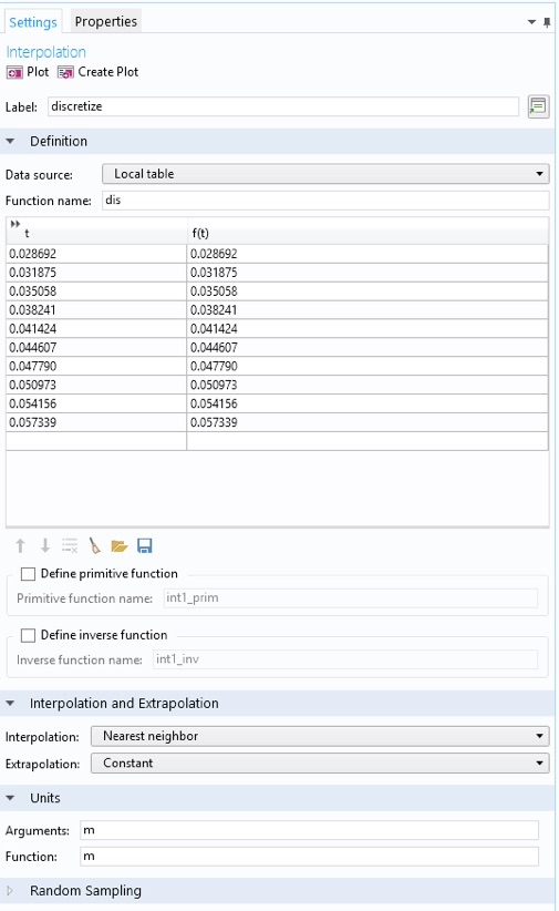
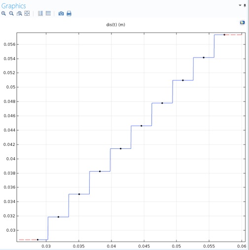
Plot the function to check it.

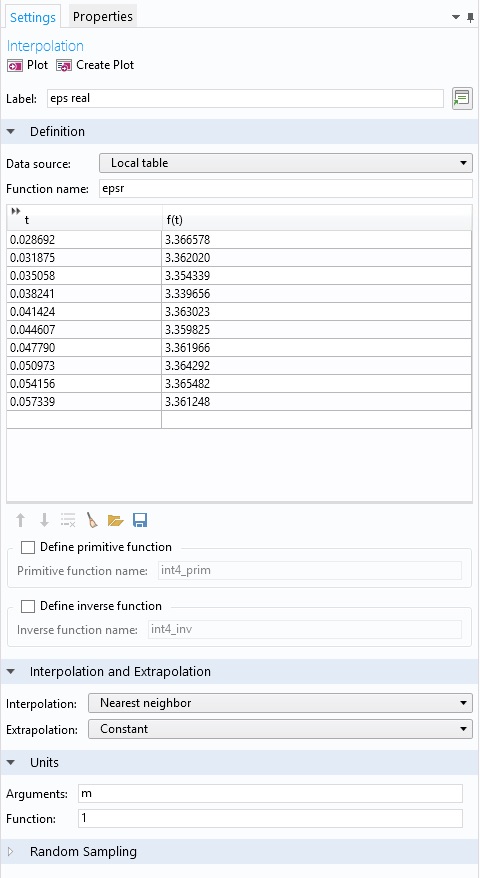
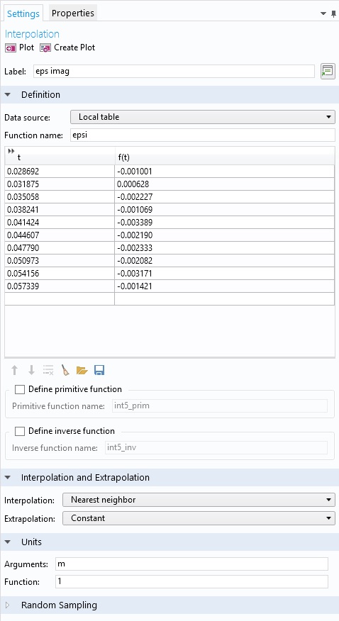
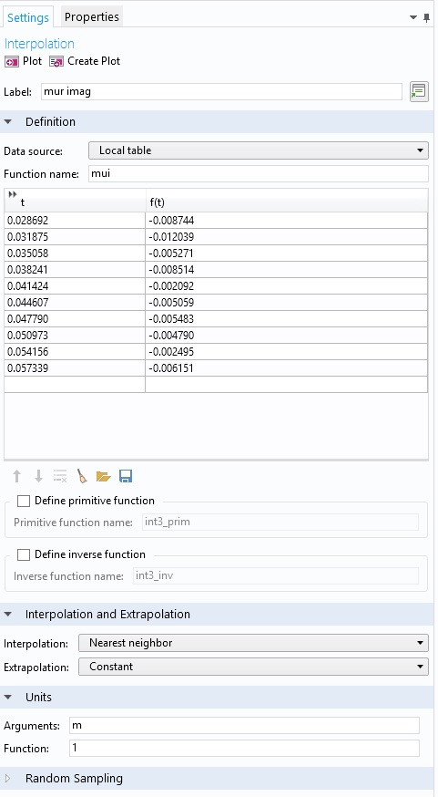
Create the four materials properties functions similarly. Note that the Function: units are, 1, dimensionless.

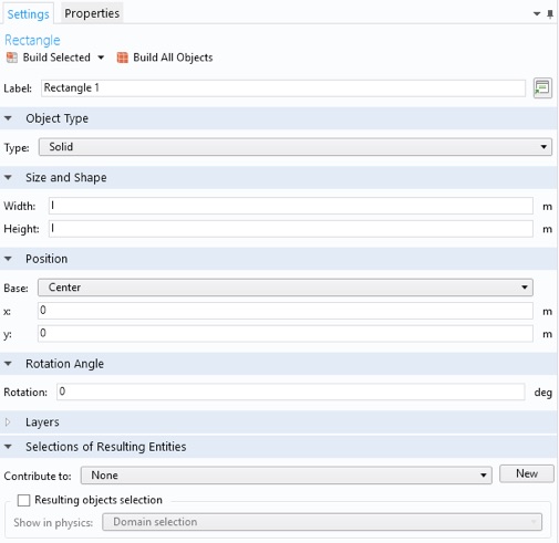
Now let’s create some geometry. First, the overall domain. Right click Geometry 1 in the Component 1 sub list. Then select Rectangle from the menu. Fill in the Width and Height using your global parameter, l , and change the Position to Center.

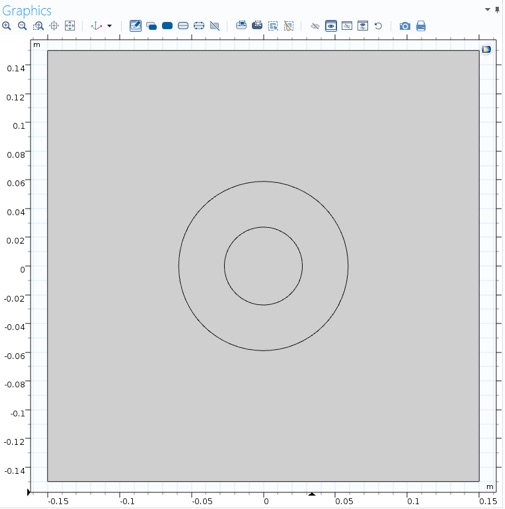
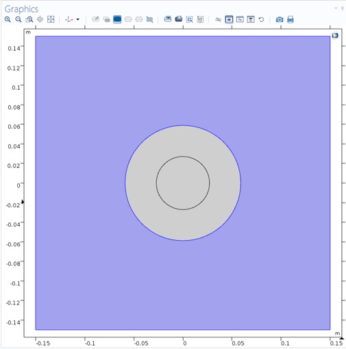
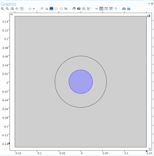
Now create the inner and outer circles of the cloak. Right click Geometry 1 and select Circle. Set the radius to the global parameter a.

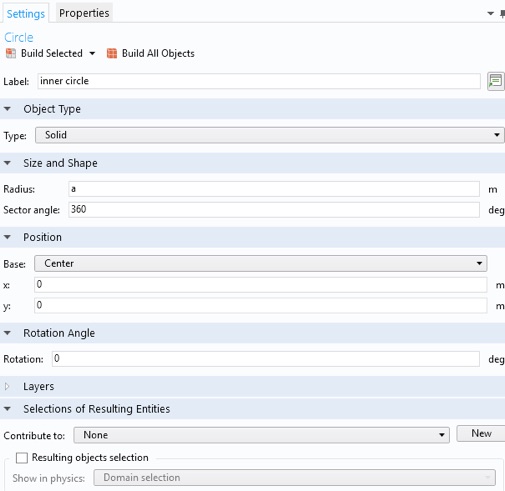
Then make the outer circle with global parameter b. Your graphics window should look like this.

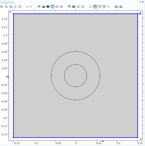
Now let’s set some boundary conditions. In the Graphics window, click the Select Boundaries item.

Then select the four outer boundaries.

Now, right click Electromagnetic Waves, Frequency Domain (emw) and select Scattering Boundary Condition. (You can also do this from the Physics tab.) The Settings pane will look like this.

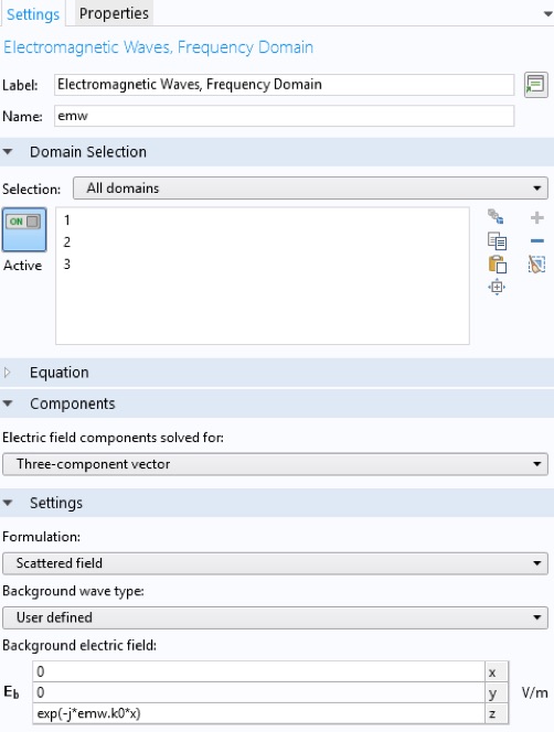
Now let’s create the incident/background field. Click Electromagnetic Waves, Frequency Domain (emw) in the Model Builder pane. In the Formulation menu, select Scattered Field. Then enter a Background electric field.

Now let’s create the material properties and assign  them to domains. Start with the space around the cloak. Right click Component 1/Materials, in the Model Builder, and select Blank Material. Fill in the background epsilonr and mur, and assign it to domain 1 (the area around the cloak). I renamed it vacuum.

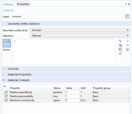
Note the highlighted domain.

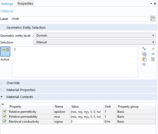
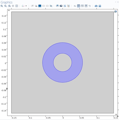
Now create the cloak material and assign it to domain 2. The epslionr and mur will be the anisotropic expression:

{ nxx, nxy, nyy, 0, 0, nz}

we will assign values to these variables later.

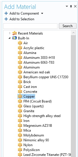
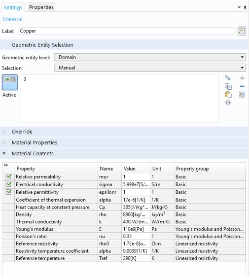
For the object to be cloaked we will use a copper cylinder (as was used in the original experiment). Right Component 1/Materials again, and select Add Material from library...

In the new pane that opens to the right, click Built-In, and then right click Copper, and select Add to Component 1.

Assign the material to domain 3, the inside of the cloak.

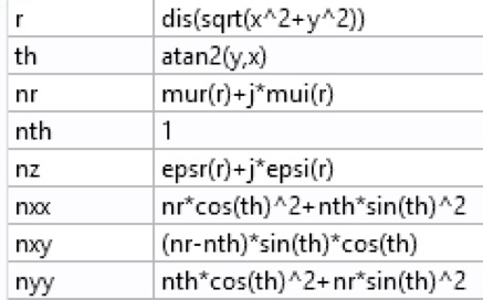
Now we will assign values to the cloak material variables for 4 different configurations. Right click Component 1/Definitions and select Variables. First create the ideal cloak configuration.

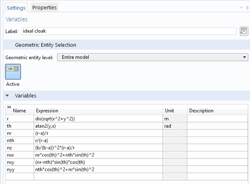
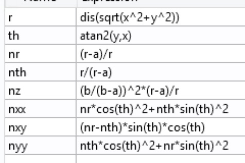
Zooming in, we see the formulas for the ideal cloak properties from the article and the formulas relating cylindrical and cartesian coordinates. The dis function (we created earlier) makes the material properties assume 10 discrete values, instead of varying continuously as a function of radius. This will be more realistic for our metamaterial cloak constructed from ten cylinders.

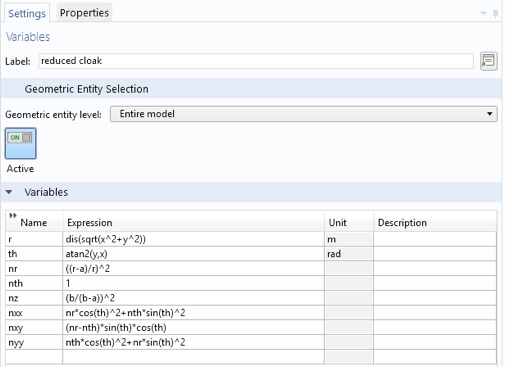
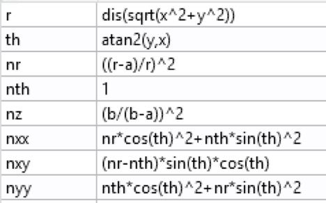
Now right click Component 1/Definitions/ideal cloak and select Duplicate. Rename this variable to reduced cloak, and input the reduced cloak properties.

Duplicate again for the metamaterial cloak.

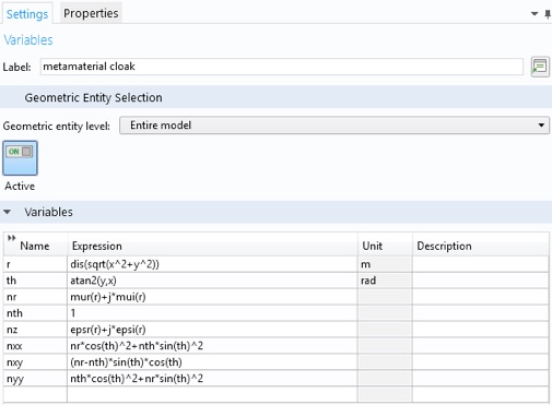
Use the interpolation functions we created from our CST data.

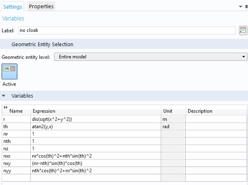
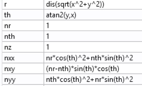
Finally, create the no cloak configuration, with vacuum properties.

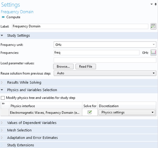
Now choose our desired frequency for the study. Select Frequency Domain under Study 1 in the Model Builder. Enter the global parameter in the Frequencies box.

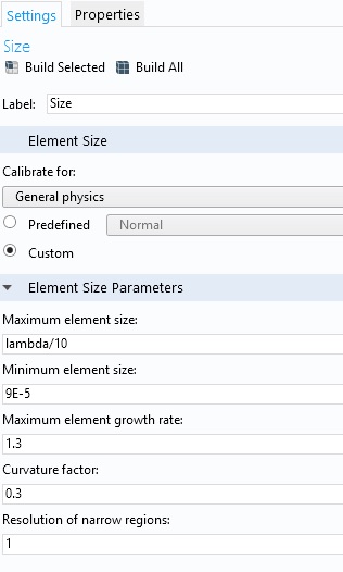
COMSOL does not know how to choose the mesh settings for our anisotropic materials. We will manually select a mesh size.

Click Component 1/Mesh 1. In the Settings tab select User-controlled mesh from the Sequence type: menu. Now click

Component 1/Mesh 1/Size. Enter lambda/10 for the Maximum element size:

You need to disable all but one of the variables under Component 1/Definitions. Do this by right clicking the variable and selecting Disable or Enable.

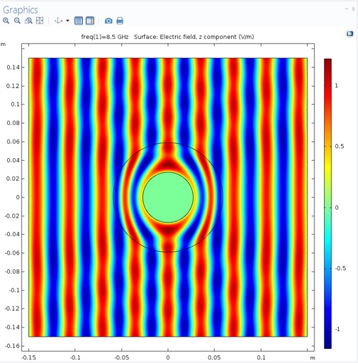
Enable just the ideal cloak variable, an then simulate. You can click Compute from: the Study tab, right-click study menu in the Model Builder, or in the Settings pane.

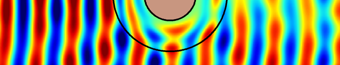
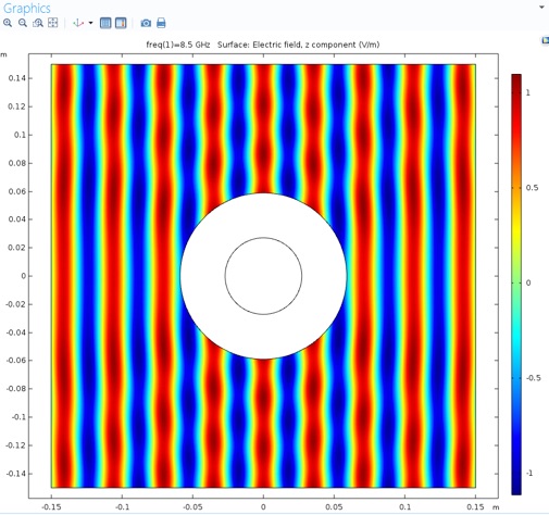
To start we will plot  the z-component of the total electric field. Click Results/Electric Field (emw)/Surface. Change the plotted expression to emw.Ez from emw.normE.

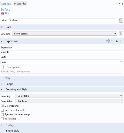
Click Plot.

4. 4.Capture this plot or for your report, and by enabling/disabling the variables, simulate, plot and capture the three other configurations for your report.
   

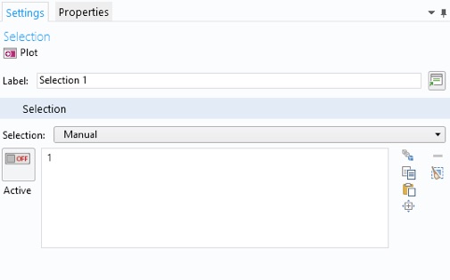
Lets look at just the scattered field. First lets omit the cloaked area from the plot (since the scattered fields there are not particularly meaningful there). Select Results/Electric Field (emw)/Surface. Then, from the Electric Field (emw) tab, click Selection, and select domain 1, the area outside the cloak. Click Plot.

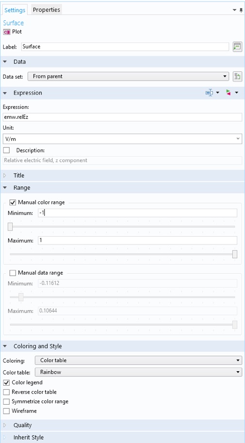
Now select Results/Electric Field (emw)/Surface again, and change the Expression to emw.relEz. Also, open the Range menu, select the Manual color range box, and enter a maximum of 1 and a minimum of -1. If you keep this range for all the scattered field plots, you will be able to make a direct visual comparison of the various configurations.

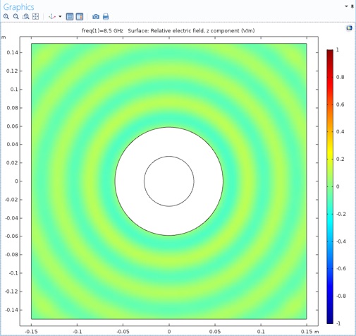
5. Capture this scattered field plot, as well as a similar plot for the other three configurations, for your report.