Assignment

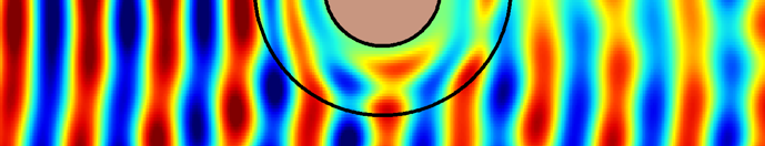
This project will examine the effects of a magnetic conducting ground plane on an antenna. We will start with a dipole antenna on a dielectric substrate, and then add magnetic and electric ground-planes, in turn.

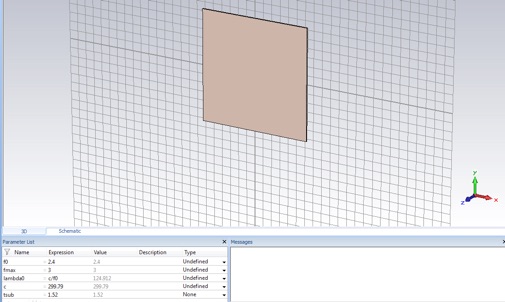
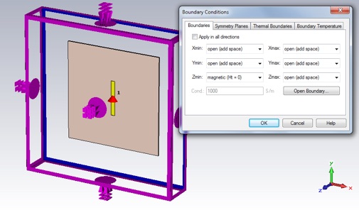
We will use a lithographically patterned dipole antenna, designed to operate at 2.4 GHz. Set the units to the usual ones (mm, GHz and ns). Set the background to Normal. Set all six boundary conditions to open (add space), and leave the Open Boundary... settings at their defaults. Set the frequency range to 0 to 4 GHz.

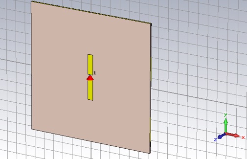
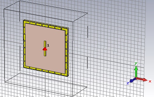
Create a square board of Rogers 3003 (lossy), using the 1.52mm thickness and side length of one wavelength at the operating frequency. Orient the board normal in the z-direction, and the bottom of the board at z = 0.

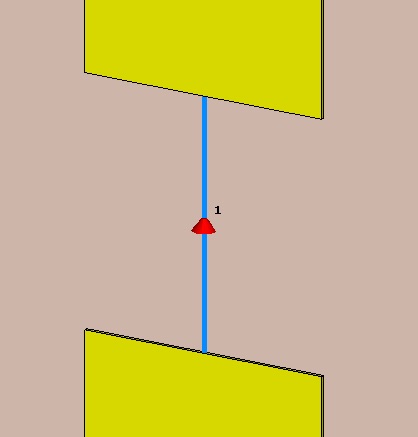
Using 2 oz copper (lossy), create a y-oriented dipole antenna that is 5mm wide, with a 5mm gap, and with length defined by a global parameter (with initial value of 1/2 operating wavelength).

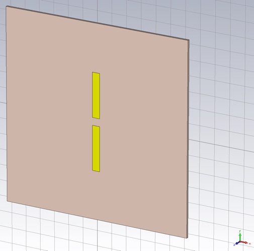
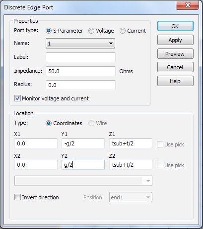
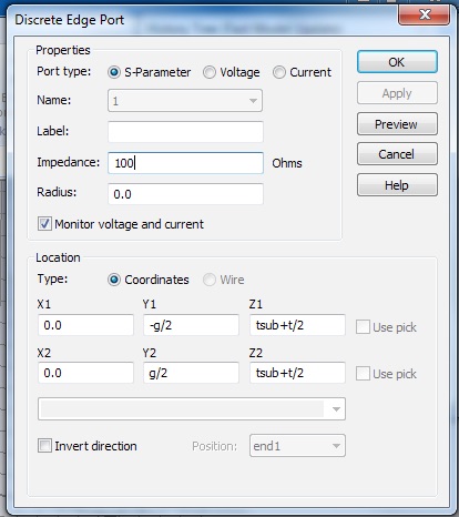
Add a discrete port to drive the antenna. Keep the impedance at 50 Ohm, which is a common standard for sources and cables.

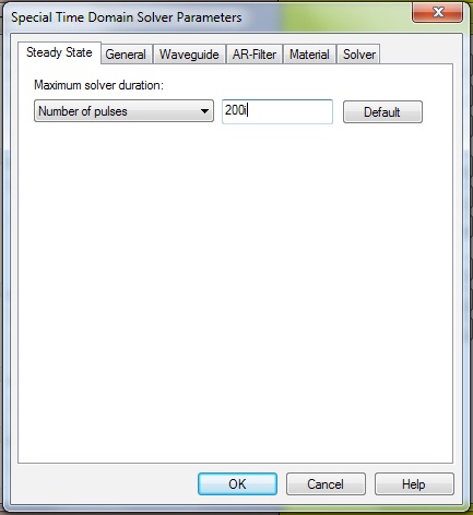
Set the accuracy to -50dB and increase the Steady State condition to a large number of pulses so that this resonant antenna will  reach this accuracy level.

Do an adaptive mesh refinement to get a suitable (converged?) mesh.

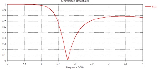
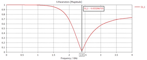
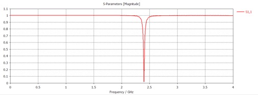
Note that the S11 dip does not occur near the desired 2.4 GHz. This is due to the substrate as well as the finite cross section of the dipole.

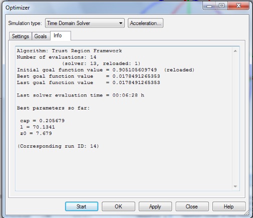
Let’s use the Optimizer to tune the antenna length. Open the Optimizer, and select your antenna length parameter for optimization. 

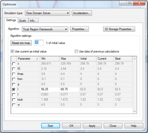
The default Min and Max values are not what we want. We know we want to raise the resonant frequency by about 1/3, so set the Min and Max values to bracket this desired change. (The range must also include the current parameter value.)

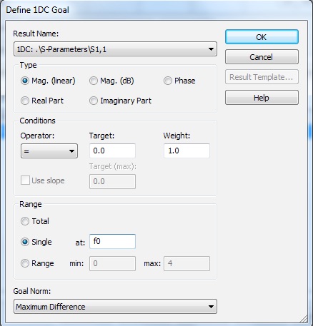
Now open the Goals tab. Adjust the goal to be a value of zero for S11 linear magnitude, at the operating frequency. (I used the variable f0 to store the operating frequency of 2.4 GHz.)

There are lots of interesting things in the Optimizer folder to watch during the optimization process. For me, it only took eight simulations to tune the antenna very precisely to the operating frequency.

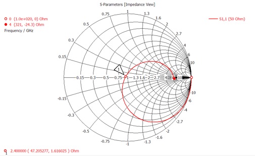
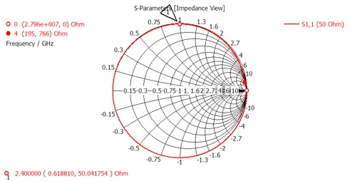
1. Place a curve marker at 2.4 GHz, and switch to the Z Smith Chart. Include this chart in your report. Is the real part of the impedance close to the source impedance? Is there a reactive part to the impedance? Is it capacitive or inductive?

Export the S11 parameter (from the polar plot, as usual, to get the full complex data). Record the optimal length.

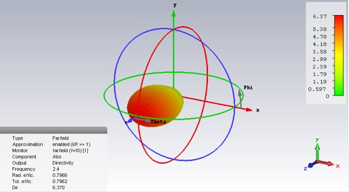
Add a Farfield monitor at the operating frequency and run the simulation again. Select your farfield folder to display a 3D plot of the antenna pattern. Select Linear scaling, and choose Directivity mode.

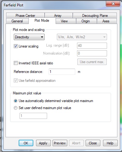
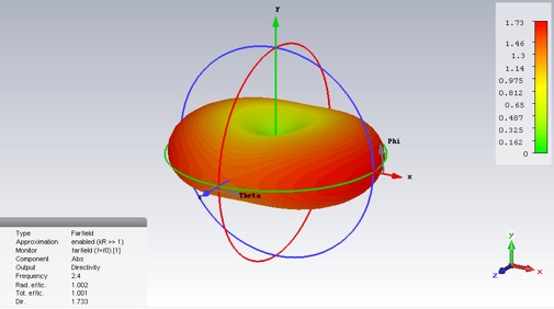
2. Get a screen grab of the 3D plot. Include the info panel (lower left) in the grab. How do the efficiency and directivity compare to what you expect?

Now add a copper (annealed) ground plane. It should cover the entire back of the substrate.

Re-run the simulation. Note that the dip in S11 is nowhere to be found in the simulated frequency range.

3. Get a screen grab of the Z Smith Chart, for your report. What is the antenna input impedance at the desired operating frequency? How does the real part of the impedance compare to standard impedances of sources and cables? Is the impedance more real or imaginary? Capacitive or inductive?

You can still match this antenna and get a strong dip in S11. By optimizing the port impedance, antenna length, and a series capacitor, I was able to obtain the results below.

The bandwidth and efficiency are terrible compared to the previous results.

Now let’s try a magnetic conducting (high impedance) ground plane. First, delete the copper ground plane. Then change the zmin boundary condition to magnetic (Ht = 0).

As discussed in class we expect this antenna configuration to have an input impedance twice that of the dipole without a ground plane. So, change the discrete port impedance from 50 to 100 Ohms.

4. 4.Compare the S11 linear plot of the optimized dipole antenna, without a groundplane, to the S11 linear plot of this antenna. Are these two antennas equally well matched?  Include a Z Smith Chart, with curve marker at 2.4 GHz, in your report. Did the impedance approximately double as expected? Include a screen grab of a 3D farfield plot. As before Select Linear scaling, choose Directivity mode, and have the info panel visible. How do the efficiencies, pattern and directivity compare to the dipole without a groundplane? Are any differences between these two, as expected?
   

Now let’s try an artificial magnetic ground plane. The basic design incorporates a unit cell with a copper patch on the front and a copper ground plane on the back. We will use 7x7 unit cells, butted up against the back of the substrate on which the antenna sits.

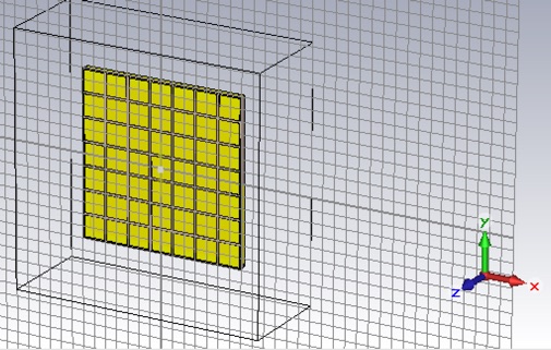
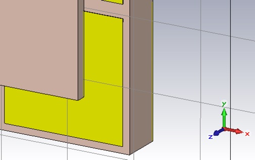
The patch and ground plane should be annealed (lossy) copper of 70 micron thickness. The ground plane substrate should be 4x1.52 mm thick, Rogers 3003. The patch should have side length of 17.8 mm with a 2mm gap between patches.

To accurately simulate this artificial magnetic ground plane we will need a finer mesh. Use a 35/35 mesh. As a result the  number of mesh nodes will be unwieldy. Use two symmetry planes to help mitigate this problem.

5. 5.Include the Z Smith Chart, and and far field plot in your report, as before. Compare the S11 dip, efficiencies, directivity and antenna pattern between the ideal PMC and the artificial magnetic conducting ground plane. What conclusions can you draw about the properties of artificial magnetic ground plane compared to the ideal PMC?