Assignment 3
Assignment
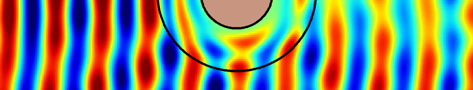
Simulate the ten different Split Ring Resonators (SRRs) in the article Metamaterial electromagnetic cloak at microwave frequencies.
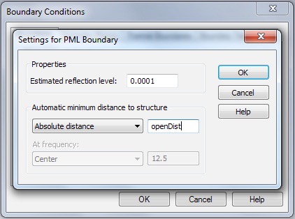
Start a new CST Microwave Studio project and do not use a template. The units we have been using (mm, GHz and nS) are probably a good choice. A frequency range of 0 to 25GHz will include the important features of the magnetic and electric resonance. The boundary conditions should be chosen so that the magnetic flux of the TEM mode links the loop of the SRR. If the SRR is oriented normal to the x-axis then the Xmin and Xmax boundaries should be magnetic. The Ymin and Ymax boundaries can then be chosen electric and the Zmin and Zmax boundaries open (add space). Select the Open Boundary... button and choose Absolute distance from the Automatic minimum distance to structure menu. You should get in the habit of using global parameters. Global parameters can be easily created by typing a valid variable name into the parameter entry fields when defining an object. You will then be prompted to enter a default value. Choose an appropriate parameter name and set the value to 3mm. You can use the variable later when you set the distance to reference plane for the ports.
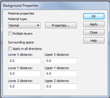
Don’t forget that the default Background Properties are PEC. Switch to Normal.
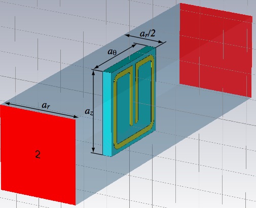
Set up the unit cell as shown below. All geometric parameters are given in the article. Use global parameters for the geometric features, r and s, in particular, since they vary for the different designs. It will also be convenient to use a global parameter for the metal thickness. (The r, θ, z subscripts here refer to the cylindrical coordinates of the cloak and not the cartesian coordinates of CST. You will probably put the ports normal to the CST z-axis.)
Start with the substrate so it will be easier to tell that the resonator ring is being located in the right place. Choose Rogers RT5870 (lossy) from the material library for the substrate and Copper (annealed) for the metal. Putting the origin at the center of the ring, and at the substrate-metal interface, may make constructing the ring easier, but other choices are fine obviously.
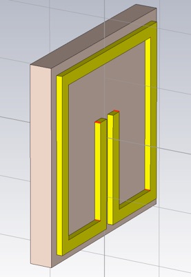
Construct the ring with square corners first then blend the edges later. You can draw a thin square slab for the ring and then cut out the center regions and gap (using appropriate bricks and boolean operations), or draw individual ring segments as bricks (making them into one object with Modeling>>Boolean>>Add). In the later case, you can use the Mirror operation under Modeling>>Transform to create half the object for you.
Now select the edges to be blended (keyboard shortcut is e then double-click the edge). Select first the edges that will have the interior radius, r (some of which are not shown below). You may want to make the object thicker to make it easier to select the edges.
Perform the blend using Modeling>>Blend>>Blend edges... Then select the edges that will have the radius, r+w (to maintain a constant cross section in the corners).
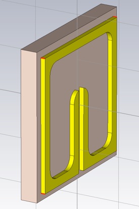
Perform the blend and return the object to its desired thickness of 0.017 mm.
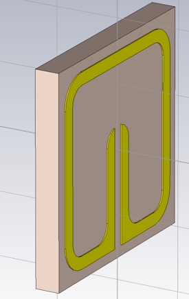
Now add some vacuum around the SRR. This should be a block that is ar by az by aθ. To resolve the intersecting shapes, you will need to trim highlighted shape for both the SRR and the substrate. You may want to make the Vacuum material transparent so you can see the SRR even when it is not selected. (Double click Materials>>Vacuum in the Navigation Tree to do this.)
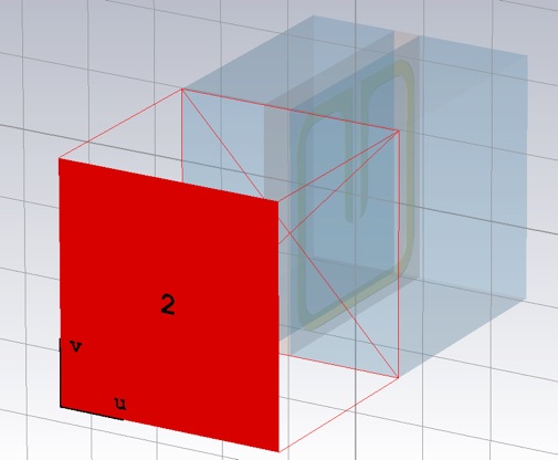
Add the ports and be sure to adjust the port reference to the edge of the substrate. (I constructed the SSR inverted here compared to the previous figures. The vertical orientation does not matter because of the mirroring action of the electric boundary conditions.)
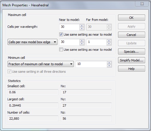
The Adaptive mesh refinement will not give a satisfactory result for reasons I will explain in class. You should use 30/30 (or higher) in the Mesh density control (Simulation>>Mesh>>Global Properties).
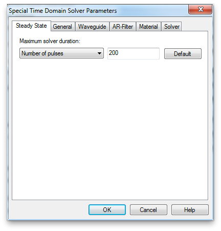
Open the Time Domain Solver Parameters, by clicking Setup Solver. As usual, use -50dB for the accuracy and set the source type to port 1 only. Click the Specials... button to bring up the Special Time Domain Solver Parameters panel. Select the Steady State tab if it is not already selected. You need to extend the steady state time out condition. The simulation will not reach the -50dB accuracy in 20 pulses. Make it 200 to ensure the simulation will run to the -50dB energy level.
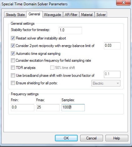
Then select the General tab. For the sharp resonances we will see in the S-parameters, it would be better to have more samples in your frequency range. Increase the Samples to 10,001. The frequency interval will then be 25GHz/10000 = 2.5 MHz. Click OK.
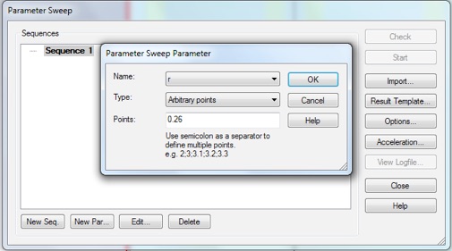
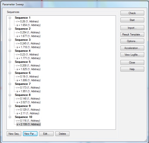
Then select Par. Sweep... to set up the simulation of all ten unit cell designs. Referencing your global parameters create a sequence for each design, adding the two parameters, r and s, with appropriate values for each.
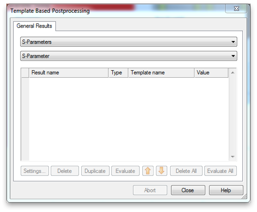
Next click the Result Template... button. Select S-Parameter from both the first and second menu.
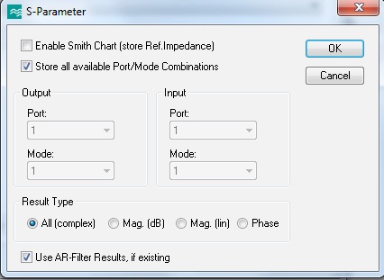
Select Store all Available Port/Mode Combinations and Result Type All(complex). Then click OK.
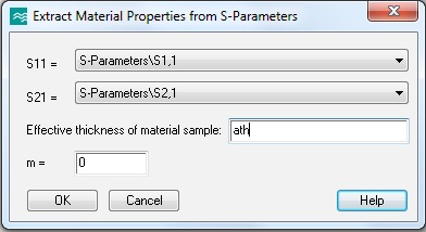
Next choose Extract Permittivity and Permeability from S-Parameters, from the second menu. Use your global parameter that defined the unit-cell thickness.
Click OK and close the Template Based Postprocessing window. Click Start in the Parameter Sweep window to begin the simulations. It might take an hour to run all ten.
Export the S-parameters. If you can export each of the two data tables to separate files, while using the Polar display, you will have all of the S-parameter data. Extract the material properties ε and μ. Note that aθ is the correct extraction thickness. You will probably not need to adjust the branch choice to obtain the correct results.
-
1.Generate a plot for ε and a plot for μ. In each, plot the real part of the ten extracted material properties versus frequency. Zoom the plot to display the region around the operating frequency, which we will take to be 8.5 GHz.
2. Also plot the real part of ε and μ versus radius, r, in the cloak at the operating frequency. The formula relating cloak radius to cylinder number is

where a is the cloak inner radius (given in the article), i is the cylinder number and ar is the radial unit cell dimension (also given in the article). In this plot versus radius, also include the desired analytical expressions for the material properties. These are given in equation (3) in the article.
-
3.An I-beam is a common metamaterial unit cell used for its providing an engineered permittivity:
Assume you have an I-beam unit cell that is well modeled by the Lorentzian

with parameters

so that at 10 GHz it provides a permittivity of

but you would like it to have a real part of permittivity of -1 and a small imaginary part. Suggest a quantitative change to make to the I-beam that will make this happen.