Assignment 6
Assignment
Start by creating a spiral unit cell that has cubic symmetry in the xz plane.
Define the usual units: mm, GHz, nS.
Load a substrate material from the library, Rogers TMM 10i (lossy).
Set the frequency range, 0 to 5 GHz.
Set the boundary conditions for a TEM mode propagating in the z direction with the magnetic field in the x direction.
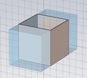
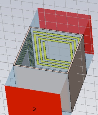
Create the substrate with thickness, ts = 0.254 mm. The substrate will be split at the unit cell boundary, so that the box shown below should have wall thickness, ts/2. (When the unit cell is periodically repeated, the substrate will have thickness ts.) The outside dimensions of the box will be that of a cube of edge length, a=5mm, the unit cell dimension. The box should probably be centered on the origin.
Create vacuum space that fills the box and extends for half a unit cell dimension beyond, in the z direction, for the ports.
Load the material, Copper (annealed) from the material library.
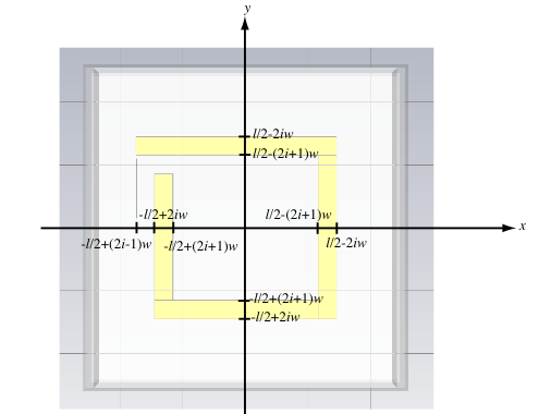
Create one loop of a spiral on the inside of one of the cube faces. The outside dimension of the spiral will be a square of edge length l=a-ts-2*w, where w=0.2mm is the trace width. The trace thickness is t=0.017mm. Define the spiral loop in terms of a spiral index, i, as shown below, so that later a multi-looped spiral can be easily created.
If you used multiple bricks to create the loop, join them all into one object with the Boolean Add command. Try changing the value of i to make sure the loop behaves as you expect it.
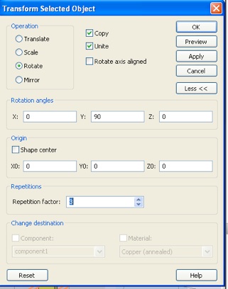
Now use the Transform Object utility to create three additional loops on each of the other faces. Be sure to check Unite, to join all the loops into a single object.
Create the ports on the z oriented faces with an appropriate reference plane shift for proper deembedding. (Probably want to save at this point.)
You should use the defaults for mesh (10/10) and accuracy (-30dB) so that the simulation will run in reasonable time. This will be important later when we do an optimization. Also, since this resonant unit cell has a fairly high Q, the excitation will not decay to this accuracy by the default steady state criteria. Increase the number of pulses from 20 to a large number like 200. While you’re at it, increase the number of frequency samples to 5001, since the default number, 1001, will be too sparse.
Open the History List in the Edit menu. Select all of the steps in the list and click Macro...
Give the macro a name. You need not make it globally available.
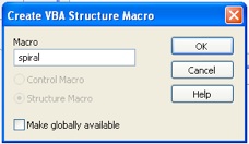
This macro will now appear at the bottom of the Macros menu. The macro script will have a tab in the work area where you can edit the macro. Click that macro tab. To save the macro (and perform many other operations) right click in the area displaying the macro script.
When you have confirmed that the macro appears in the Macro menu and see that it contains all the steps from your model, you can delete all the steps in the history list and click update. Now select your macro in the Macro menu to recreate your unit cell.
While you debug your script you will frequently have to remove any objects it creates so that you can run the script again without conflicts between existing objects and objects the script is creating. One way to do this is to delete any items in the history list and click update. This will return you to a clean slate.
You should become familiar with the CST VBA language reference.
Put a For loop around the commands that: create your spiral bricks, add the bricks together, and rotate them onto the four faces of you unit cell. You will need to declare an index variable i to replace the global index i you used in constructing the model. Put a Dim statement just below the declaration of the script Main subroutine.
Sub Main ()
Dim i As Integer
The For loop syntax is:
For i = 0 To n-1
statements
Next i
You should remove the global parameter i from your list. You want the script to refer to your loop variable when creating the bricks. One way to do this is to remove the quotes around any command arguments that refer to i. (I hope there is another way, but I do not know of it.)
Create a global parameter n to set then number of windings in the spiral, with a value of three to start with. Run the script and see if generates three windings. Debug it.
You also need to modify the script so that the first time through the loop the connecting tab is not created. My code looks like this:
With Brick
.Reset
.Name "spiral"+Str(i)
.Component "component1"
.Material "Copper (annealed)"
If i>0 Then
.Xrange -l/2+(2*i-1)*w, l/2-(2*i)*w
Else
.Xrange -l/2+(2*i)*w, l/2-(2*i)*w
End If
.Yrange l/2-(2*i+1)*w, l/2-(2*i)*w
.Zrange -a/2+ts/2, -a/2+ts/2+t
.Create
End With
Note also the argument to Name. You need to create a unique name each time through the loop to avoid conflicts. (The three other bricks in your winding do not need unique names since you are adding those bricks to this one, and they then no longer exist.)
To make all three windings into a single object you can put another Add command at the bottom of your For loop:
If i>0 Then Solid.Add "component1:spiral 0", "component1:spiral"+Str(i)
Now when you run the macro you should have a single object that comprises four, three winding, spirals on each inside cube face of the unit cell. Run the transient solver to make sure the model is working.
1. Submit your structure macro.
It would be nice to calculate the effective medium properties from inside CST instead of having to export the the S-parameters to perform the extraction. This would make it possible to use CST optimization for obtaining specific material property goals.
You can add your own Template Based Postprocessing calculations by creating scripts and storing them in the appropriate file location. I have created this script which you can store here:
C:\Program Files\CST STUDIO SUITE 2011\Library\Result Templates\S-Parameters
This script will then appear in the bottom menu when select S-Parameters from the top menu of the Template Based Postprocessing panel. Try running it.
This script has most of the VBA language constructs you will need to make a template for extracting material properties from the S-parameters and storing the result in the Navigation Tree.
Some notes on this script. You will probably want to use a number of real valued variables for intermediate results. You should dimension these as doubles, for example:
Dim x, y, u, v, r, s As Double
I did not use the macro editing tools or debugger for this script, but you can if you want to. (I don’t know how this will work out, since the result template scripts are called by CST with some framework in place.) You can just use any text editor, store the script in the appropriate directory and run the script from the Template Based Postprocessing panel. In this regard, it is important to know that you must delete and re-add your script to the processing list to have changes you have made to the script take effect.
The big challenge is to do this complex calculation without native complex mathematical operations. To do this you need the rules that specify how the relevant complex valued functions’ real and imaginary parts are computed using real valued functions, for example:
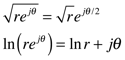
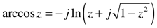
Or, you could access this information using Mathematica’s ComplexExpand function, or to a lesser extent Matlab’s real and imag functions. (An alternative approach would be to find a VBA library that implements complex math, perhaps this one.) The arccos function is a bit tedious and Matlab cannot do it for you, so here is the VBA code for it, complements of Mathematica:
re( arccos( r + i s ) )
Pi/2.-ATn2(r+(4*r^2*s^2+(1-r^2+s^2)^2)^0.25*Sin(ATn2(-2*r*s,1-r^2+s^2)/2.),
-s+(4*r^2*s^2+(1-r^2+s^2)^2)^0.25*Cos(ATn2(-2*r*s,1-r^2+s^2)/2.))
im( arccos( r + i s ) )
Log(Sqr((-s+(4*r^2*s^2+(1-r^2+s^2)^2)^0.25*Cos(ATn2(-2*r*s,
1-r^2+s^2)/2.))^2+(r+(4*r^2*s^2+(1-r^2+s^2)^2)^0.25*Sin(ATn2(-2*r*s,1-r^2+s^2)/2.))^2))
You will also need the material thickness, d, in your calculation. There are several ways to obtain this value for your script. For example, you can reference the global parameter variable that you used to create your unit cell, or you could get the distance between the port 1 and port 2 reference planes from a CST VBA object.
2. Write and submit Template Based Postprocessing scripts that extract the complex refractive index and impedance from the S-parameters and store them in the Tables folder of the Navigation Tree (one script for n and one for Z).
3. Provide plots of the imaginary part of n and Z calculated using your scripts. How many discontinuities are there in each of these plots?
These discontinuities are of course removable by proper branch correction. Fortunately, you need not do this by hand. Your scripts can amended to handle the choice of branch. Here are some code snippets for that purpose.
For the n script, inside the loop on frequency, you can use this code
xp = x + Round((x0-x)/(2*Pi))*2*Pi
yp = y
xm = -x + Round((x0+x)/(2*Pi))*2*Pi
ym = -y
If (x0-xp)^2+(y0-yp)^2 < (x0-xm)^2+(y0-ym)^2 Then
x = xp
y = yp
Else
x = xm
y = ym
End If
x0 = x
y0 = y
where x and y are assumed to contain the real and imaginary parts of inverse cosine (from the code above). Before your frequency loop you will need to initialize the values of x0 and y0
x0 = 0.01
y0 = 0
For the Z script, inside the loop on frequency, you can use this code
If (x0-x)^2+(y0-y)^2 > (x0+x)^2+(y0+y)^2 Then
x=-x
y=-y
End If
x0=x
y0=y
where x and y are assumed to contain the real and imaginary parts of the square root, and the intialization for x0 and y0 is
x0=1
y0=0
Of course, you will also need to declare all the new variables as doubles.
4. Provide plots of the imaginary part of n and Z calculated with your amended script that does branch correction. Have the discontinuities been removed?
Add Postprocessing template items to calculate the permittivity (eps) and permeability (mu) from n and Z.
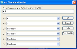
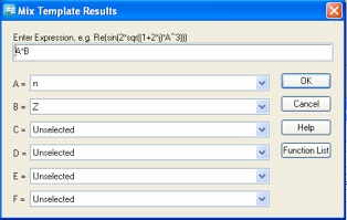
You may want to name these results appropriately.
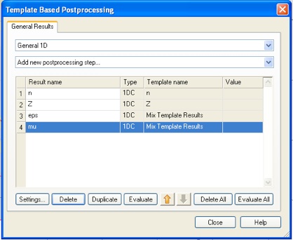
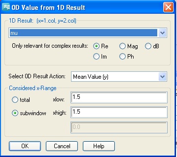
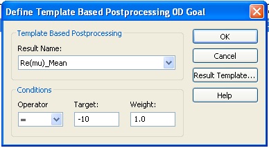
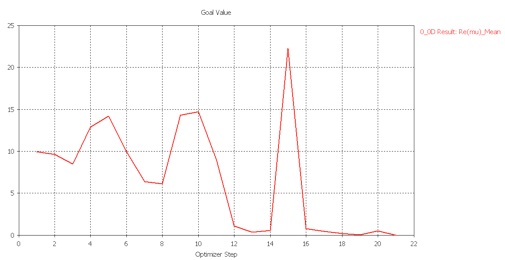
Now we can optimize the structure to obtain a particular value of a material property at a particular frequency. We will try to find a unit cell structure with a permeability of -10 at a frequency of 1.5 GHz. Add a 0D result to the Postprocessing list.
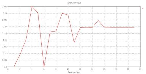
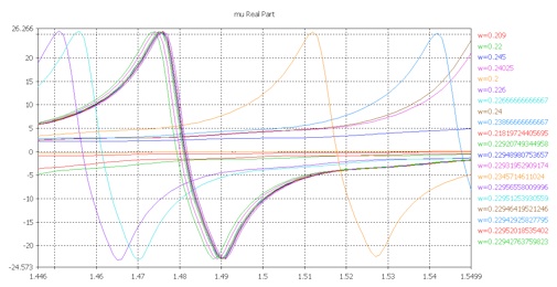
Set up the optimizer. We will vary the trace width, w. The range 0.2 to 0.25 mm should work. Set a fairly tight domain accuracy so that the optimized result will be accurate even though the slope of the mu curve is steep. (Use 0.0001 not the value shown below.) A local optimizer algorithm is probably best for this narrow single parameter search. When you move on to the Goals tab CST will warn you that there is no dependence on the parameter w, but we know better. (The w dependence of the structure is in the macro.)
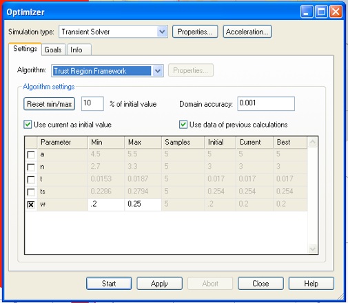
From the Goals tab, set a goal for the real part of mu.
Before starting the optimizer you might want to confirm that you are using the default mesh (10/10) and accuracy (-30dB). The individual simulations should take less than 5 minutes.
5. For the optimized unit cell, report the complex value of mu and eps at 1.5 GHz. How does the tan-delta of the effective mu and epsilon compare with that of the substrate material we used, TMM-10i? (Recall that tan-delta is the imaginary part divided by the real part, and for the refractive index, gives a measure of wave attenuation per unit wavelength.)
Solution
-
2.These scripts do not do branch correction:
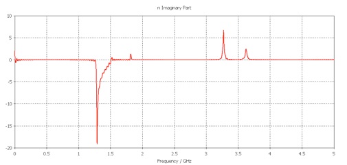
3.Imaginary part of the refractive index:
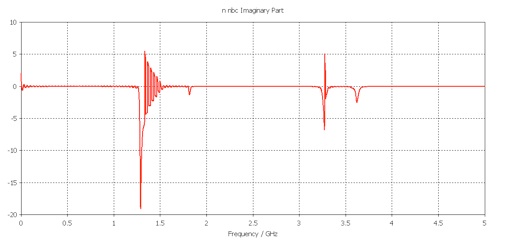
Zoom to see the discontinuities:
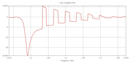
It looks like thirteen discontinuities in the refractive index.
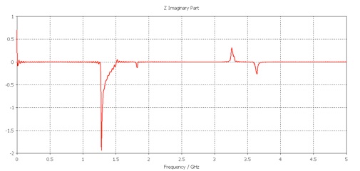
Imaginary part of the impedance:
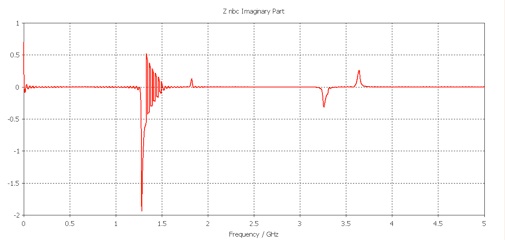
Zoom to see the discontinuities:
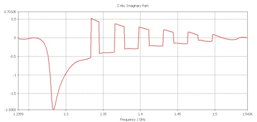
It looks like eleven discontinuities in the impedance.
These scripts do do branch correction:
-
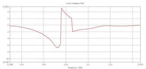
4.Imaginary part of the refractive index, branch corrected:
Imaginary part of the impedance, branch corrected:
The discontinuities have been removed.
The optimization settles on w = 0.2294 mm.
-
5.With the optimized width, w, and at the desired frequency:
eps = 11.573+0.021j
mu = -10.000-0.539j
and the tan deltas:
|Im(eps)/Re(eps)| = 0.002 (gain)
|Im(mu)/Re(mu)| = 0.054
The imaginary part of eps is positive, due to spatial dispersion, aka the anti-resonance. For comparison, the substrate eps tan delta is 0.002, which is much smaller than the effective mu tan delta. (There is a price to be paid for this unusual material property.)