Assignment 5
Assignment
We will start simulating a half-wave dipole antenna. Create two identical cylinders of lossy Aluminum along the z-axis with a gap between them. (They should be centered on the origin so you can use symmetry planes to speed up the computation.) Create a box of space (vacuum) around the antenna. Set the frequency range to include the operating frequency, maybe 0 to 3 GHz.
Operating center frequency: 1.96 GHz (middle of the GSM1900 downlink band)
Antenna end-to-end length (starting): half wavelength at the operating frequency, lambda/2
radius: 1.5 mm
gap: 3mm
x space: -lambda/4 to +lambda/4
y space: -lambda/4 to +lambda/4
z space: -lambda/2 to +lambda/2
Add a discrete port that spans the gap and is parallel to the z-axis. Set the global mesh properties so that there are more than two mesh intervals across the diameter of the antenna cylinders.
Set the boundary conditions to open on all boundaries. Use all three symmetry planes. Choose magnetic or electric for each symmetry plane to match the properties of the fields driven by the discrete port.
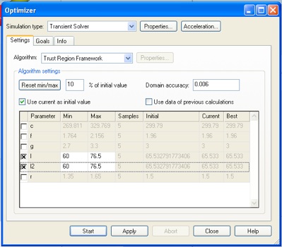
Run the simulation with an accuracy of -50dB. Is the minimum of S11 at the operating frequency? If not use the optimizer to adjust the length of the antennas so that the S11 minimum lies at the operating center frequency. You should set the range of the antenna length parameter so that it goes down to 60 mm or so. You should also reduce the the domain accuracy to find the optimal length to within 0.1 mm. (Any more precision is unnecessary and takes more simulation time.) Since there is only one dip in the S11 spectrum (for our frequency range), a local optimization algorithm is should be more efficient.
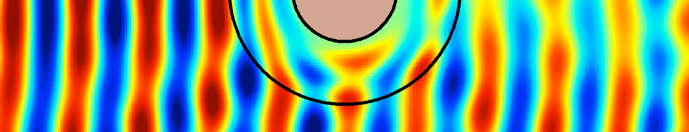
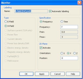
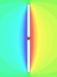
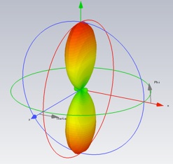
Now add a far-field monitor at the operating center frequency and re-simulate using the optimized length. Also add an H field monitor so we can verify the current distribution is in fact what we expect for a half wave dipole. Set this monitor also the operating center frequency and activate the 2D plane (either x or y).
Run the transient solver.
0. Provide a Smith chart for S11, with the operating frequency tagged with a curve marker. Note the proximity of the impedance at the operating frequency to the port impedance.
Check that the component of field normal to the 2D plane has the expected mode shape.
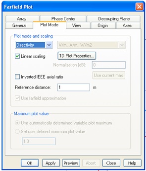
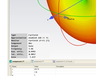
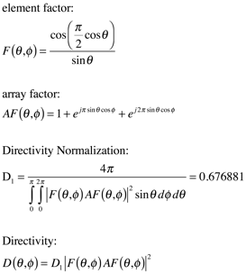
Now look at the far fields. Select Farfields>>farfield in the Navigation tree. Now select Farfield Plot Properties from the contextual menu. If you check Linear scaling in the Plot Mode tab, the plot and the numerical efficiencies will be given in linear units.
-
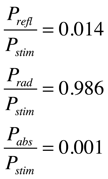
1.As in assignment 4, report the reflected, radiated and absorbed power. (In this case there is no power transmitted to another port.) Was the absorbed power less than you expected? Why do you think it’s so low?
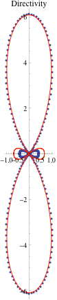
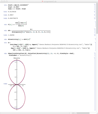
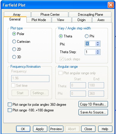
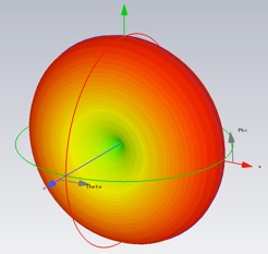
Now we want to export the directivity to compare with a theoretical dipole. Select Directivity in the Plot Mode tab and select Polar and Theta in the General tab. (Since the antenna is complete symmetric in the phi direction, so is the directivity. There is no need to look at the phi dependence.)
Export the data. Note that the directivity is labeled Abs(Gain) in the resulting text file.
-
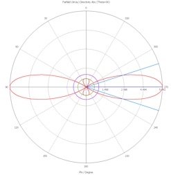
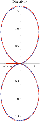
2.Plot the directivity data in linear polar form together with the theoretical directivity of a half-wave dipole antenna. Can you suggest a reason why the directivity might differ from the theoretical result?
The directivity of a half-wave dipole antenna is given in section 2.2 of Stutzman and Thiele or section 4.6 of Balanis.
Use CST’s array factor capability to predict the far-field for a three element array. From the farfield results, bring up the Farfield Plot panel and select the Array tab. Select Antenna array and open the properties panel. Make a three element array along the x-axis with a Spaceshift of lambda/2 (half the wavelength at the operating frequency) and a Phaseshift of zero (i.e. a broad side array).
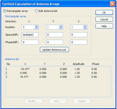
Note the drastic change in the antenna pattern.
Display and export the phi dependence of the directivity with theta equal to 90 degrees.
-
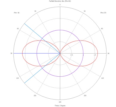
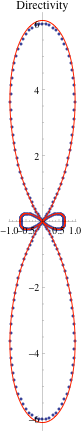
3.Plot this directivity data in linear polar form together with the theoretical directivity of the array (including both the theoretical half-wave element and the theoretical array factor.)
Now simulate the real three element array. Add two more elements to the array with positions as above. Note that their are now two unique environments for the array elements: center and end. You will need to be able to tune both element types separately. Define a new length variable and use it to construct elements surrounding the original element. Recreate the space block so that it extends beyond the array by lambda/4 in all directions. Also, add discrete ports for each of the new elements.
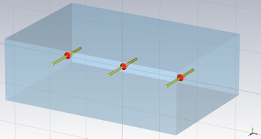
Note that one of the symmetries has been spoiled and the symmetry plane will need to be removed. In fact the simulation will not run until you do.
Run the simulation, with type of All Ports.
-
4.Has the S11 minimum shifted? Are the minima of S22 and S33 the same as S11? Report the location (i.e. the frequency) of the minima of S11, S22 and S33.
Now try to optimize the array for matched operation. We will do this by maximizing Pin1 and Pin2. (Pin3 has the same numerical value as Pin2.)
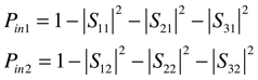
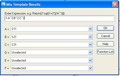
Enter all the relevant S-parameters in the Template Based Postprocessing panel, and add Pin1 and Pin2 and 0D entries for Pin1 and Pin2 at the operating frequency.
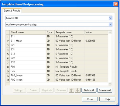
Pin1 will look like this.
Now open the optimizer and choose the antenna length parameters. You can use the same range as before.
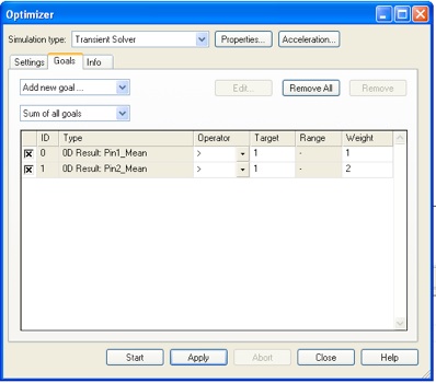
Add your 0D Pin goals. Since there are two elements with the input power of Pin2, set the weights accordingly.
Since only S-parameters with port 1 and port 2 excited are needed for the goal function, you can speed up the optimization by using Selection for the excitation type and choosing only those ports. Now run the optimization.
5. Find the distribution of power (Prefl, Ptrans x2, Prad, Pabs) separately for each type of excitation, the middle port and and end port.
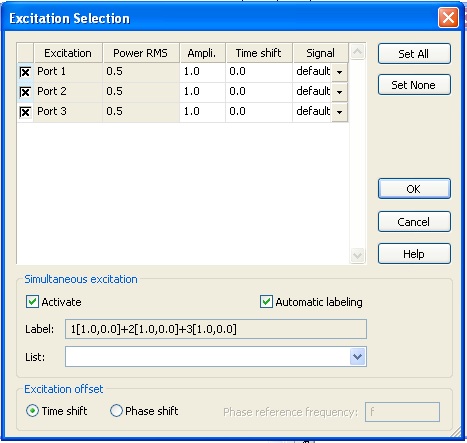
Make sure the optimal lengths are set for the all the elements and simulate with simultaneous excitation of all three of the ports. Open the Excitation List from the Transient Solver panel and check Activate in the Simultaneous excitation area. Leave the default amplitude and time shift. Since we want our array to be driven in phase, there is no time shift. Click OK an then Start.
Again plot the phi dependence of the directivity at theta equals 90 degrees, making sure the array factor is deactivated (i.e. select Single antenna). Export the data.
-
6.As in 3 above, plot this directivity data in linear polar form together with the theoretical directivity of the array (including both the theoretical half-wave element and the theoretical array factor.) Now that we have simulated real elements in a real array, is the agreement with theory worse than in 3, where we had a real element and an ideal array factor?
Solution
0. Note that the curve marker placed at the operating frequency (1.96GHz) is the point of closest approach to one, the reference impedance of the Smith chart. The marker impedance is 61.8-5.5j Ohm.

1. The antenna length that minimizes S11 at the operating frequency is 65.533mm. At this length and frequency the power distribution is (to three decimal places):
2.
3.
-
4.Due to coupling, the three minima are now at frequencies different than the desired operating frequency. (All three antennas have length 65.533mm as above.):
S11: 2.037 GHz
S22: 2.010 GHz
S33: 2.010 GHz
-
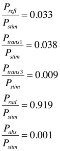
5.The optimal lengths I found were l(center) = 68.037 and l(end) = 67.481. With these lengths and at the desired operating frequency (1.96 GHz), the power distribution for center excitation was:
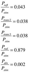
For end excitation:
6.