Simulation of the Frequency Domain Reflectometer in ADS
Introduction
The Frequency Domain Reflectometer (FDR) is used to determine the length of a wire. By analyzing data collected from this simple circuit we can determine the condition of the wire under test. This tutorial will focus on how to setup and simulate the FDR under a variety of circumstances. We will start by creating a new project and setting up the actual FDR circuit. This design will then be used to analyze different wire configurations.
FDR Setup
From the Main window (Fig. 1) in ADS select a new project by selecting File and then New Project, or click the folder icon to the far left of the tool bar. Name the project when prompted, and then a blank design page should appear. We are now ready to create our FDR circuit.
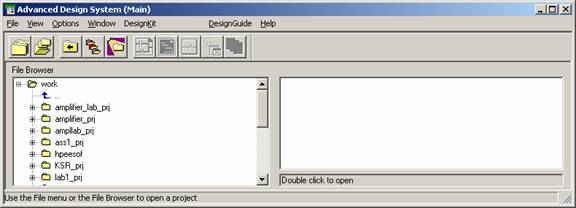
Fig 1. ADS Main Window
We will be creating the circuit shown in Fig 2. We start by placing the Voltage source to the left. This part can be found in the Sources-Freq Domain Library. Libraries are selected in the pull-down menu to the far left of the screen. Make sure that all
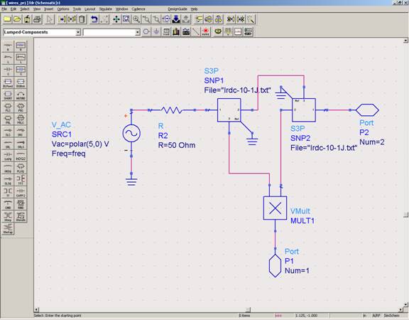
Figure 2. FDR circuit.
settings are as shown in the figure. Parameters can be altered by double clicking the component itself, or by single clicking the parameter, and typing the value to be changed.
Next we place the Resistor, which can be found in the Lumped-Components Library. To rotate a part simply press ‘Ctrl-R’ while the part is selected.
Three-port S-Parameter boxes in the middle represent the couplers. These cannot be found in a Library. Instead we place the cursor in the pull-down menu next to the one for the libraries. We then type ‘s3p’. When we move the cursor back to the design page we see the three-port S-Parameter box. These should be placed as shown. Remember to rotate the second one as shown. Next we double click on the component. This will produce another dialog box. Select the ‘File’ Option and then select ‘Browse’ next to the box that displays the name of the file. You can then select the name of the S-Parameter file that represents the couplers being used. This file should be placed in the ‘Data’ folder of the project. For more information on how to set up these files consult the ADS documentation. Appendix A contains the file used in this example.
The VMult acts as our mixer. It can be found in the System-Amps & Mixers Library. Double click on the component and select the linear parameter. Change this to ‘yes.’
Ports can be found to the right of the popup-menus. Place the first port on the bottom, and the second one at the upper right. Ports will allow the circuit to function within other more complex systems without redrawing the entire circuit.
Ground connections are to the immediate left of the Port connections. Place these as shown in the circuit.
Finally we connect the parts with wires. Wires are drawn by typing ‘Ctrl-W’ and clicking on the nodes we wanted connected. We can also move a part until one node touches the other, and then sliding it back into position.
Finally we save this figure by selecting the disk icon. Name it ‘FDR.’ We are now ready to move onto more complex wire systems.
Wire Setup
The previous section established a basic FDR design, and serves as a template for all future simulations. It can be simply copied and pasted into a new project, where it can be developed and simulated as desired. This section will discuss what can be done with the FDR once it has been placed in a project.
First we discuss some things that will need to be in place for all simulations. After we have setup the FDR as described in the previous section we select File, New in the design window. This opens a new design window where we can perform the simulation. First we need to place the MSUB parameters. This is found in the TLines-Microstrip Library. This will provide the characteristics of all the MLINs which we will use to represent our wires. Figure 3 shows some sample values that could be used for this. Figure 3 also shows the values that should be used for the AC simulation parameters. The values shown are the same used in the FDR200. Thie can be found in the Simulation AC Library.
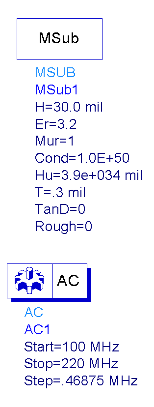
Figure 3 Parameter values for MSUB and AC Simulation
The simplest simulation one might perform is a single straight wire. The wire will be simulated by a microstrip line titled MLIN. This part can be found in the TLines-Microstrip Library. The length and impedance can be changed based on the values entered for length and width, respectively. For the MSUB parameters shown in Figure 3 a width of 71.695 mils corresponds to a 50 W Transmission Line. Notice that the length does not have to be in the same units of measurement. All other values should be left as default.
To add the FDR we type ‘FDR’ in the same box we used earlier to obtain the Three-Port S-Parameter box. The part will then appear. Port one should be connected to the transmission line, and port should have a wire connected to it that terminates a short distance from the FDR as shown in Figure 4. This wire should be named by clicking the red icon labeled name on the second row of the design window.
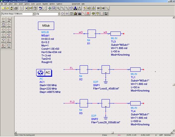 Figure 4.
Single wires connected to FDR.
Loss can be modeled through two-port S-Parameter boxes. These are obtained in the same manner as the ‘S3P’ blocks used in the FDR circuit. Type ‘S2P’ in the same block, insert them between the FDR and the wire, and then specify the file to be used.
More complex wiring diagrams can be obtained by using the MTEE found in the same library as the MLIN. This acts as a T-Connector between wires, and allows complex branches to be created.
We are finally ready to simulate! This can be done by pressing F7, selecting the ‘yellow gear’ icon next to the name icon, or by selecting Simulate, Run. From the menu bar. This will produce the window shown in Figure 5, as well as a blank data display similar to that shown in Figure 6. In the Data Display Window, click on the ‘square graph’ icon immediately below the ‘arrow’ icon on the right. This will produce the graph shown in Figure 6 with a window prompting for the data to be displayed. This dialog box is shown in Figure 7. The names of wires labeled by the user will appear. Select the one you would like displayed, then select ‘>>Add>>.’ The dialog box shown in Figure 8 will appear. Select ‘Magnitude’, then click ‘OK.’ Click ‘OK’ again. This will then display data similar to that shown in Figure 6.
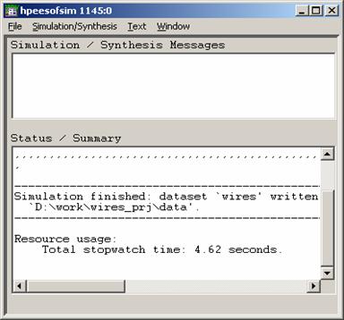
Figure 5. Simulation Results Report
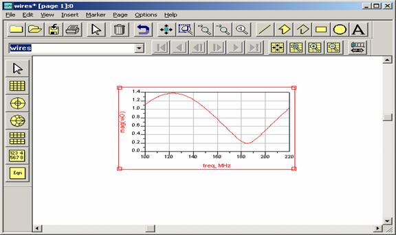 Figure 6.
Data Display Window.
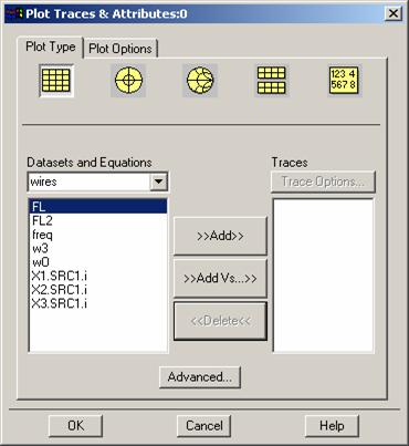
Figure 7. Data Display Dialog Box.
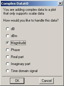
Figure 8. Data Display sub Dialog Box
Finally we need to process the data. A simple FFT function is available in ADS, however better results, including additional processing can be obtained in Matlab. A sample program that performs this analysis is found in Appendix B. To export the data from ADS we select File, Export, Write selected item to tab-delimited ASCII. This is shown in Figure 9. In order for this option to be available the data display box must be selected (A red box will surround the graph). Once the file has been exported. The first line must be deleted, and the file needs to be moved to the Matlab path to be processed.
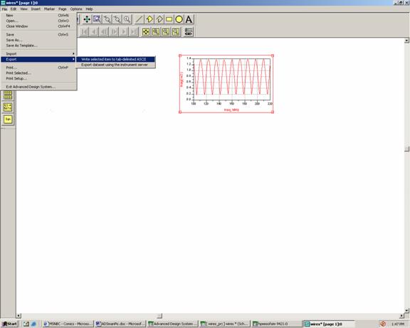
Figure 9. Export data to text file.
Appendix A
Three-Port S-Parameter File
Click above to open (Right click to save)
Appendix B
M-File to Analyze ADS DATA
Click above to open (Right click to save)